ECN 102: Analysis of Economics Data

Homework 3 Answer Key

Author

Remy Beauregard

Question 1: Bivariate model assumptions

What is the first population assumption of bivariate OLS regression? How might this assumption be violated? How could we account for this violation?

Linearity: the true relationship between x and y is linear. This could be violated if we instead have a true nonlinear relationship, which we could account for by adapting our regression to match.

What is the second population assumption of bivariate OLS regression? How might this assumption be violated? How could we account for this violation?

Unbiasedness: the conditional expected value of our error term is zero for all values of x. This could be violated if there are variables missing from our regression that are correlated with x and y. We could address this by including these missing/omitted regressors in a multivariate regression.

What is the third population assumption of bivariate OLS regression? How might this assumption be violated? How could we account for this violation?

Homoskedasticity: the distribution (variance) of our errors is constant across values of x. This could be violated if the distribution of our errors changes for larger or smaller values of x. We could account for this by using robust standard errors in our regression.

What is the fourth population assumption of bivariate OLS regression? How might this assumption be violated? How could we account for this violation?

Independence: our error terms are uncorrelated for different units of observation. This could be violated if our observations are not independent from each other, such as time-series data of GDP for a given country. We could account for this by using more complicated forms of regression that account for error dependence.

Question 2: Manual calculations

Consider a dataset with 3 observations for $(x,y): (2,4),(1,3)$ and $(6,2)$.

From first principles (using formulas not Stata), compute:

the OLS intercept

$x_i$	$y_i$	$\bar{x}$	$\bar{y}$	$(x_i-\bar{x})$	$(x_i-\bar{x})^2$	$(y_i-\bar{y})$	$(y_i-\bar{y})^2$	$(x_i-\bar{x})(y_i-\bar{y})$
2	4	3	3	−1	1	1	1	−1
1	3	3	3	−2	4	0	0	0
6	2	3	3	3	9	−1	1	−3

\[b_1=\bar{y}-b_2\bar{x}=3-\left(-\frac{4}{14}\right)\times3=\boldsymbol{3.86}\]

the OLS slope coefficient

\[b_2=\frac{\sum_i(x-\bar{x})(y-\bar{y})}{\sum_i(x-\bar{x})^2}=\frac{-1+0-3}{1+4+9}=-\frac{4}{14}=\boldsymbol{-0.29}\]

residuals for the three observations

\[e_i=y_i-\hat{y}_i:\]

\[\begin{aligned} 4-[3.86-0.29\times2] &= 4-3.28 = \boldsymbol{0.72} \\ 3-[3.86-0.29\times1] &= 3-3.57 = \boldsymbol{-0.57} \\ 2-[3.86-0.29\times6] &= 2-2.12 = \boldsymbol{-0.12} \end{aligned}\]

\[\sum_i e^2_i = 0.86\]

the $R^2$ of reg y x (or reg x y)

\[R^2=1-\frac{\sum_i e_i^2}{\sum_i(y_i-\bar{y})^2}=1-\frac{0.86}{2} = \boldsymbol{0.57}\]

the covariance of X and Y

\[Cov(x,y)=\frac{\sum_i(x_i-\bar{x})(y_i-\bar{y})}{n-1} = \frac{-1 + 0 - 3}{2} = \boldsymbol{-2}\]

the correlation between X and Y

\[r_{xy} = \frac{Cov(x,y)}{s_xs_y} = \frac{-4}{\sqrt{14}\sqrt{2}} = \boldsymbol{-0.76}\]

Question 3: Bivariate regression

Use AED_SALARYSAT.DTA.

What variables are present in our dataset? List them along with their labels.

u AED_SALARYSAT, clear
des

(Data for A. Colin Cameron (2022), ANALYSIS OF ECONOMIC DATA, Amazon)

Contains data from AED_SALARYSAT.dta
 Observations:           876                  Data for A. Colin Cameron
                                                (2022), ANALYSIS OF ECONOMIC
                                                DATA, Amazon
    Variables:            12                  22 Jan 2022 15:50
-------------------------------------------------------------------------------
Variable      Storage   Display    Value
    name         type    format    label      Variable label
-------------------------------------------------------------------------------
salary          float   %9.0g                 Annual Salary in dollars
lnsalary        float   %9.0g                 Natural Logarithm of Annual
                                                Salary
satverb         int     %32.0g                SAT test verbal score (highest
                                                self-reported score as of 2007)
satmath         int     %32.0g                SAT test mathematics score
                                                (highest self-reported score as
                                                of 2007)
highgrade       byte    %8.0g                 Highest grade ever completed
age             float   %9.0g                 Age in years
sex             byte    %14.0g                1 = female 0 = male
minority        float   %9.0g                 1 = minority 0 = not minority
height          float   %9.0g                 Height in inches
weight          int     %8.0g                 Weight in pounds
genhealth       byte    %9.0g                 Health status: 1=Excellent
                                                2=VeryGood 3=Good 4=Fair 5=Poor
actscore        float   %32.0g                ACT test score (highest
                                                self-reported score as of 2007)
-------------------------------------------------------------------------------
Sorted by:

Suppose we want to run a regression of salary on SAT verbal score. Perform this regression and interpret the output.

reg salary satverb


      Source |       SS           df       MS      Number of obs   =       876
-------------+----------------------------------   F(1, 874)       =      9.61
       Model |  5.7575e+09         1  5.7575e+09   Prob > F        =    0.0020
    Residual |  5.2357e+11       874   599052503   R-squared       =    0.0109
-------------+----------------------------------   Adj R-squared   =    0.0097
       Total |  5.2933e+11       875   604947912   Root MSE        =     24476

------------------------------------------------------------------------------
      salary | Coefficient  Std. err.      t    P>|t|     [95% conf. interval]
-------------+----------------------------------------------------------------
     satverb |   23.92566   7.717525     3.10   0.002     8.778612    39.07271
       _cons |   23752.62   4278.621     5.55   0.000     15355.05     32150.2
------------------------------------------------------------------------------

$\boldsymbol{\widehat{salary}=23752.62+23.93\times SATverb}$. Variation in SAT verbal score accounts for 1.09% of variation in salary.

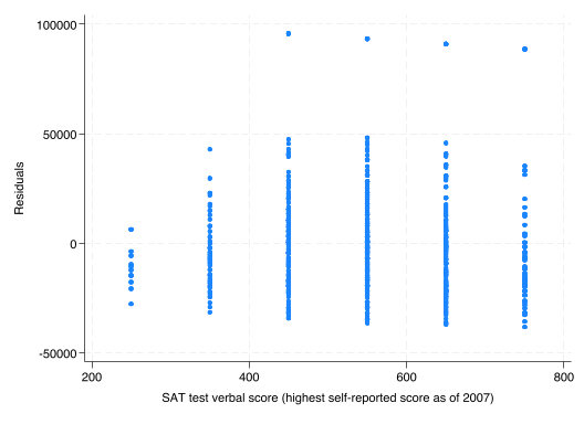
Generate the residuals from the above regression using predict resid, resid and plot these against SAT verbal scores in a scatter plot. Do our errors appear to be homoskedastic or heteroskedastic?

predict resid, resid
sc resid satverb

Our errors appear to be a bit heteroskedastic, with larger errors for larger values of SAT verbal score.

Make changes to the regression in part (b) to account for your answer in part (c). How does this change your estimated coefficients? How does this change your estimated standard errors? Does this make sense?

reg salary satverb, robust


Linear regression                               Number of obs     =        876
                                                F(1, 874)         =      10.30
                                                Prob > F          =     0.0014
                                                R-squared         =     0.0109
                                                Root MSE          =      24476

------------------------------------------------------------------------------
             |               Robust
      salary | Coefficient  std. err.      t    P>|t|     [95% conf. interval]
-------------+----------------------------------------------------------------
     satverb |   23.92566   7.454351     3.21   0.001     9.295139    38.55618
       _cons |   23752.62   3922.598     6.06   0.000     16053.81    31451.44
------------------------------------------------------------------------------

We would want to add the , robust option to our regression to account for this heteroskedasticity. This should change our standard errors but not our point estimates for our coefficients. In this case, robust standard errors decrease our standard error and increase our t-score for our slope coefficient.

Question 4: Bivariate regression

Using AED_CALELECTRICITY.DTA from hw2, we now want to investigate when electricity gets more and less expensive.

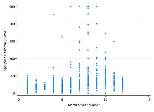
Create a scatterplot of the spot price of electricity and the month. What do you notice?

u AED_CALELECTRICITY, clear
sc niso month

(Data for A. Colin Cameron (2015): Analysis of Economics Data, W.W. Norton)

We notice that the spot price of electricity is higher and more varied during the summer months.

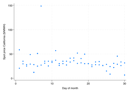
Create a scatterplot of the spot price and the day only for the month of November. What do you notice?

sc niso day if month==11

We notice that there is an outlier value of around $150 for the spot price on one day, and that otherwise the spot price is relatively consistent.

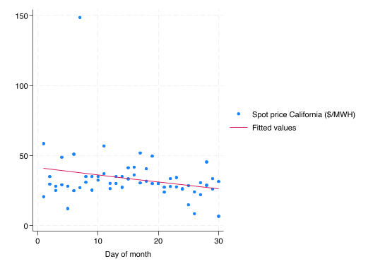
Overlay a best fit line onto your scatterplot from part (b). Without calculations or running a regression, what would you expect $b_1$ and $b_2$ to be for a regression of day on spot price in the month of November?

sc niso day if month==11 || lfit niso day if month==11

We would expect a $b_1\approx40,b_2<0$ given what we see from the best fit line.

Between day and month, which series is more correlated with the spot price?

corr niso month day

(obs=682)

             |     niso    month      day
-------------+---------------------------
        niso |   1.0000
       month |   0.1685   1.0000
         day |   0.0345   0.0309   1.0000

Month is more correlated with niso than day (0.1685 vs. 0.0345).

Perform the regression from part (b) of the spot price on day during November. Interpret your results.

reg niso day if month==11


      Source |       SS           df       MS      Number of obs   =        60
-------------+----------------------------------   F(1, 58)        =      3.63
       Model |   1142.9022         1   1142.9022   Prob > F        =    0.0617
    Residual |   18260.543        58  314.836949   R-squared       =    0.0589
-------------+----------------------------------   Adj R-squared   =    0.0427
       Total |  19403.4452        59  328.871953   Root MSE        =    17.744

------------------------------------------------------------------------------
        niso | Coefficient  Std. err.      t    P>|t|     [95% conf. interval]
-------------+----------------------------------------------------------------
         day |  -.5042428   .2646537    -1.91   0.062    -1.034005    .0255192
       _cons |   41.28264    4.69838     8.79   0.000     31.87781    50.68747
------------------------------------------------------------------------------

We see that indeed our intercept term is near 40 and our slope is negative: electricity prices decrease throughout November.

Suppose we are concerned our data violates the third assumption of bivariate linear regression. What could we add to part (e) to address this? Make this change and interpret your new results.

If we are worried that our data violates homoskedasticity, we can add the , robust option to our regression to accommodate heteroskedastic errors.

reg niso day if month==11, robust


Linear regression                               Number of obs     =         60
                                                F(1, 58)          =       3.26
                                                Prob > F          =     0.0761
                                                R-squared         =     0.0589
                                                Root MSE          =     17.744

------------------------------------------------------------------------------
             |               Robust
        niso | Coefficient  std. err.      t    P>|t|     [95% conf. interval]
-------------+----------------------------------------------------------------
         day |  -.5042428   .2792251    -1.81   0.076    -1.063173     .054687
       _cons |   41.28264   6.187393     6.67   0.000     28.89723    53.66806
------------------------------------------------------------------------------

What would we expect the spot price of electricity to be on the first day of November? On the last?

$\boldsymbol{41.28-0.50\times1=\$40.78}$

$\boldsymbol{41.28-0.50\times30=\$26.28}$

Find a day of the month in November with a positive residual. Find a day of the month in November with a negative residual.

predict residual if month==11, resid
list day residual if month==11

(622 missing values generated)

     +-----------------+
     | day    residual |
     |-----------------|
215. |   1    -20.2084 |
216. |   2   -10.77416 |
217. |   3   -11.75792 |
218. |   4   -10.26567 |
219. |   5   -10.74923 |
     |-----------------|
220. |   6   -13.38402 |
221. |   7   -10.75294 |
222. |   8   -6.391131 |
223. |   9   -11.50615 |
224. |  10   -3.870217 |
     |-----------------|
225. |  11    1.264027 |
226. |  12    -5.15282 |
227. |  13    .2725123 |
228. |  14   -6.953245 |
229. |  15   -.4112209 |
     |-----------------|
230. |  16     2.88871 |
231. |  17   -2.319207 |
232. |  18    -.578613 |
233. |  19   -1.742032 |
234. |  20   -1.257788 |
     |-----------------|
235. |  21   -3.400575 |
236. |  22   -2.397103 |
237. |  23      4.5078 |
238. |  24   -3.319216 |
239. |  25   -.2365738 |
     |-----------------|
240. |  26   -4.223382 |
241. |  27    2.844042 |
242. |  28    1.516274 |
243. |  29    6.748436 |
244. |  30    5.244639 |
     |-----------------|
580. |   1    17.73547 |
581. |   2   -5.362309 |
582. |   3   -14.76754 |
583. |   4    9.423758 |
584. |   5   -26.75543 |
     |-----------------|
585. |   6     12.6519 |
586. |   7    110.8419 |
587. |   8   -2.248702 |
588. |   9   -1.753259 |
589. |  10   -1.249295 |
     |-----------------|
590. |  11     21.0517 |
591. |  12    -8.95045 |
592. |  13   -4.726318 |
593. |  14    .7754047 |
594. |  15    7.505836 |
     |-----------------|
595. |  16    8.373722 |
596. |  17    19.04674 |
597. |  18    8.315207 |
598. |  19    17.80392 |
599. |  20   -1.197088 |
     |-----------------|
600. |  21   -6.910365 |
601. |  22    3.276666 |
602. |  23   -2.148201 |
603. |  24   -2.899697 |
604. |  25   -13.92638 |
     |-----------------|
605. |  26   -19.77889 |
606. |  27   -5.686239 |
607. |  28      18.177 |
608. |  29    -.658703 |
609. |  30   -19.59514 |
     +-----------------+

Interpret the t-stat, p-value, and confidence interval for $b_2$ in your regression from part (f). What test does this correspond to? What are its hypotheses? What is its conclusion and why?

This is our test of association between day and niso. \[H_0:\beta_2=0;\quad H_A:\beta_2\neq0\] With $\alpha=0.05$, we fail to reject the test of association as our p-value is 0.076>0.05. We can also confirm this conclusion with our critical value approach or our confidence interval including 0.

\(x_i\)	\(y_i\)	\(\bar{x}\)	\(\bar{y}\)	\((x_i-\bar{x})\)	\((x_i-\bar{x})^2\)	\((y_i-\bar{y})\)	\((y_i-\bar{y})^2\)	\((x_i-\bar{x})(y_i-\bar{y})\)
2	4	3	3	−1	1	1	1	−1
1	3	3	3	−2	4	0	0	0
6	2	3	3	3	9	−1	1	−3

Other Formats

Question 1: Bivariate model assumptions

Question 2: Manual calculations

Question 3: Bivariate regression

Question 4: Bivariate regression