(obs=69)

             |    price      mpg   weight    rep78
-------------+------------------------------------
       price |   1.0000
         mpg |  -0.4559   1.0000
      weight |   0.5478  -0.8055   1.0000
       rep78 |   0.0066   0.4023  -0.4003   1.0000
ECN 102: Analysis of Economics Data
Chapter 10: Multivariate Regression
Remy Beauregard
Course Logistics
A reminder to fill out course evaluations:
https://eval.ucdavis.edu/
Let us know what works well and what we can improve — all feedback is appreciated!
We also have our Stata quiz this week during Thursday section — please review Mitali’s Canvas announcement and plan to arrive on time. The exam is 50 minutes. Hw 1-3 AKs will be available.
Those taking through SDC will receive an email from me at their scheduled exam time with alternate submission instructions.
Motivation for Multivariate Regression
Previously, we modeled and conducted inference on the relationship between two variables, X and Y. However, we are likely to encounter many scenarios where we think more than one explanatory variable is important for explaining an outcome variable. In this case, we need to utilize multivariate regression.
Challenges of Multivariate Regression
Multivariate regression is a bit more complicated than bivariate:
We cannot produce a scatterplot in more than 2 (or 3) dimensions, meaning we may not easily be able to visualize our series together in a single plot.
We also cannot compute correlation between more than two variables, meaning our statistics will be a bit more complicated.
We may think that some regressors covary with others, meaning we will need to work harder to isolate the unique contribution each regressor makes to changes in our outcome variable.
Pairwise Correlations
We may still want to think about correlation between variables in the multivariate case, but we are restricted to two variables at a time. Instead, we may compute and display a set of pairwise correlations: how each variable of interest varies with all other variables individually. We have seen an example of this in Stata:
The Multivariate Regression Model
Our multivariate regression model will look quite similar to the bivariate model but with additional terms: \[\hat{y}=b_1+b_2x_2+b_3x_3+...+b_kx_k\]
where \(\hat{y}\) is our outcome or dependent variable and \(x_2...x_k\) are our \(k-1\) independent variables or regressors. \(b_2...b_k\) are then the estimated coefficients associated with each regressor.
Our \(i^{th}\) observation will be given as \(\hat{y}_i=b_1+b_2x_{2i}+...+b_kx_{ki}\).
Residuals in Multivariate Regression
Just like bivariate regression, our residual is the vertical distance between our actual and fitted values: \(e_i=y_i-\hat{y}_i\), which can now be expanded to \[e_i=y_i-\underbrace{(b_1+b_2x_{2i}+b_3x_{3i}+...+b_kx_{ki})}_{\hat{y}_i}\]
However, we need to know how to estimate the \(k\) unknown coefficients in our regression model, \(b_1,...,b_k\)
Normal Equations (First-Order Conditions)
Our \(k\) OLS coefficients are found as the solution to \(k\) first order conditions or normal equations set equal to zero: \[\sum_{i=1}^nx_{1i}(y_i-b_1-b_2x_{2i}-...-b_kx_{ki})=0\] \[\sum_{i=1}^nx_{2i}(y_i-b_1-b_2x_{2i}-...-b_kx_{ki})=0\] \[...\] \[\sum_{i=1}^nx_{ki}(y_i-b_1-b_2x_{2i}-...-b_kx_{ki})=0\]
We obtain these by applying the chain rule to \(\frac{\partial}{\partial b_j}\sum_i e_i^2\) for \(j=1,...,k\).
Orthogonality
Given our definition of our residual as \(e_i=y_i-\hat{y}_i\) and our normal equations above, we can rewrite these FOCs as \[\sum_{i=1}^nx_{ji}e_i=0\text{ for }j=1,...,k\] We see that this means the sum of the products of each regressor and the residual is zero, also called orthogonality.
Since we know that our constant term means \(x_{1i}=1\) for all \(i\), we can show that \(\sum_ie_i=0\) for OLS: \[\sum_{i=1}^nx_{1i}e_i=0\rightarrow\sum_{i=1}^n1e_i=0\rightarrow\sum_{i=1}^ne_i=0\]
Perfect Collinearity
An additional constraint on our multivariate regression is that our regressors are not perfectly collinear with each other (or with linear combinations of each other). For example, if we had a regressor \(x_2=3x_3\), we could not include both \(x_2\) and \(x_3\) in our multivariate regression.
Even if our regressors are not perfectly collinear, we may still be concerned if two or more of our regressors are highly (but not perfectly) correlated.
Since we are solving \(k\) FOCs to find \(k\) unknown coefficients, we also need to ensure that our sample size exceeds our number of regressors: \(n>k\)
Estimating Coefficients: The Formula for \(b_j\)
Unlike bivariate regression, we cannot easily express a complete formula for our coefficient estimates.
If we consider \(b_j\) to be the coefficient on the \(j^{th}\) regressor in a multivariate regression, our coefficient will be equal to the ratio of the covariance (with our residual) to the variance of the residual of a regression of \(x_j\) on all other regressors:
\[b_j=\frac{\sum_{i=1}^n\tilde{x}_{ji}(y_i-\bar{y})}{\sum_{i=1}^n\tilde{x}_{ji}^2}=\frac{Cov[\tilde{x}_j,y]}{V[\tilde{x}_j]}\]
where our residual \(\tilde{x}_{ji}=x_{ji}-\hat{x}_{ji}\) and \(\hat{x}_{ji}\) is the predicted value of \(x_{ji}\) from a regression of \(x_j\) on all other regressors \(x_{j'\neq j}\).
Implications of the \(b_j\) Formula
Given our formula, we can see that:
\(\tilde{x}_{ji}=x_{ji}-\bar{x}_j\) if \(x_j\) is independent of all other regressors
\(\tilde{x}_{ji}=x_{ji}-\bar{x}_j\) if \(x_j\) is our only regressor (bivariate regression)
\(\tilde{x}_{ji}=0\) if \(x_j\) is perfectly collinear (exactly overlaps) with one or more other regressor \(x_{j'\neq j}\) in our model
In cases (1) and (2), we see that \(b_j=b_j^{\text{bivariate}}\) when we plug in \(\tilde{x}_j\).
In case (3), we see that \(\tilde{x}_j=0\) will mean we cannot estimate \(b_j\) as we will have a zero in our denominator.
Overlapping Variation: Diagram
Variation of \(x_j\) overlapping with other regressors:
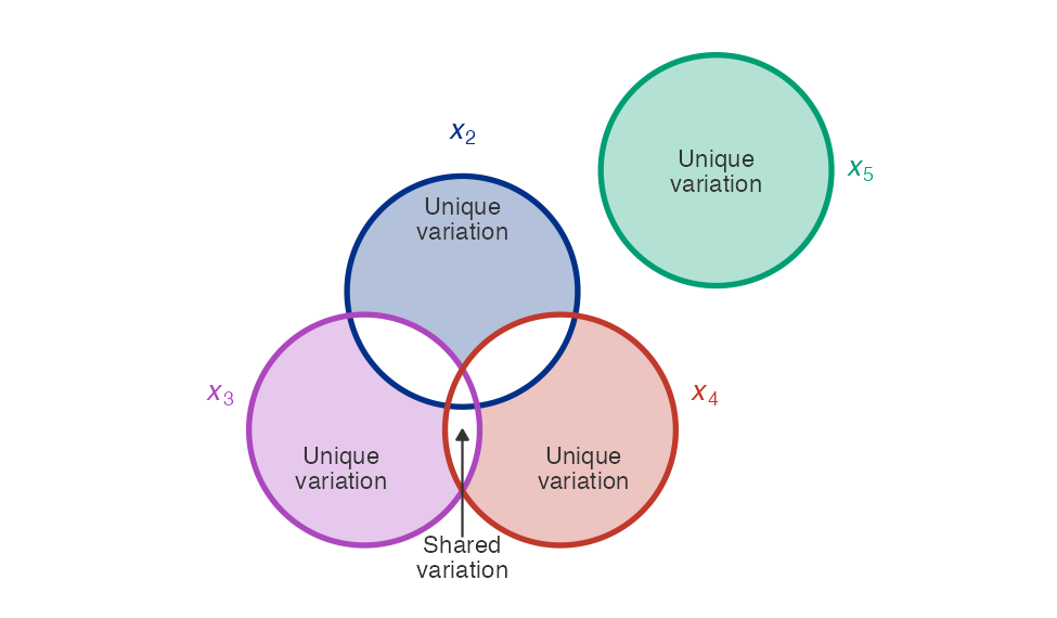
Total variation of each regressor (full circle) and the unique variation used for OLS estimation (shaded non-overlapping region).
Why Unique Variation Matters
Why do we need to identify unique variation of \(x_j\), \(\tilde{x}_j\)?
Suppose we want to estimate the associated change in \(y\) when \(x_2\) changes: this is our coefficient \(b_2\). However, we also know that \(x_2\) and \(x_3\) are correlated and both appear in our regression1.
Now, suppose we observe that:
\(x_2\) increases
\(x_3\) increases
\(y\) increases
Did \(y\) increase because \(x_2\) changed? Or did \(y\) increase because \(x_3\) changed and \(x_2\) changed because it is correlated with \(x_3\)? If variation in \(x_2\) and \(x_3\) (or any regressors) is allowed to overlap, we must identify the unique contribution \(x_2\) makes to changes in \(y\).
Example: Estimating Coefficients in Practice
What would this look like in practice? Suppose we want to estimate: \[final_i=\beta_1+\beta_2MT_i+\beta_3StataQuiz_i+\beta_4\overline{HW}_i+\beta_5\overline{KC}_i+u_i\] for your grade on the final as a function of your other grades in this class. How would we estimate \(\beta_3\), the coefficient on StataQuiz?
First, we would regress StataQuiz scores on all other regressors. Then, we would find the residuals of this regression. Finally, we would compute the ratio of the covariance of \(x_3\) residuals with the residuals from our main regression to the variance of \(x_3\) residuals.
Partial Effect vs. Total Effect: Definitions
There are two effects from our regressor \(b_j\) we might be interested in: the partial effect or the total effect
The partial effect is the impact on our outcome variable when \(x_j\) changes and all other regressors are held constant.
The total effect is the impact on our outcome variable when \(x_j\) changes and we allow all other regressors \(x_{j'\neq j}\) that may covary with \(x_j\) to change and impact our outcome variable through their associated coefficients.
It follows that the partial effect will be equal to the total effect if our regressor \(x_j\) is independent from all other regressors \(x_{j'\neq j}\).
Partial and Total Effects: Formulas
We express the partial effect as: \[\frac{\partial\hat{y}}{\partial x_j}=b_j\]
We express the total effect as: \[\begin{align*} \frac{d\hat{y}}{d x_j} &= \underbrace{\frac{\partial\hat{y}}{\partial x_j}}_{b_j}\underbrace{\frac{\partial x_j}{\partial x_j}}_1+\sum_{j'\neq j}\underbrace{\frac{\partial\hat{y}}{\partial x_{j'}}}_{b_{j'}}\frac{\partial x_{j'}}{\partial x_j} \\ &= \underbrace{b_j}_{\text{direct effect}}+\underbrace{\sum_{j'\neq j}b_{j'}\frac{\partial x_{j'}}{\partial x_j}}_{\text{indirect effect(s)}} \end{align*}\]
Total Effect Equals Bivariate Coefficient
With some math, we can also show that the total effect of \(x_j\) in a multivariate regression of y is equal to the \(b_2\) coefficient from a bivariate regression of y on \(x_j\).
This should make sense: the total effect is the direct effect of \(x_j\) on y plus any indirect effects through other variables. The sum of these effects must then be equal to the effect of \(x_j\) on y alone in a bivariate regression.
Stata cannot automatically compute the total effect of \(x_j\) for us using the regress command (more advanced commands are required), but we can compute it by hand using the formula above.
Model Fit in Multivariate Regression
Luckily, our measures of model fit do not need to change much to accommodate multivariate regression, since they depend on our residual (\(e=y-\hat{y}\)):
RMSE: \[s_e=\sqrt{\frac{1}{\boldsymbol{n-k}}\sum_{i=1}^n(y_i-\hat{y}_i)^2}\]
\(R^2\) \[\frac{ExpSS}{TSS}=\frac{\sum_{i=1}^n(\hat{y}_i-\bar{y})^2}{\sum_{i=1}^n(y_i-\bar{y})^2}\left[=1-\frac{ResSS}{TSS}\right]\]
Notice: we now have \(n-k\) degrees of freedom in our RMSE denominator, since we are estimating coefficients on \(k\) regressors (instead of two) to use in our calculation.
The Problem with \(R^2\)
Unhelpfully, our \(R^2\) will always weakly increase as we add regressors1, but we may face other downsides to endlessly adding regressors to our model.
We therefore might want to introduce a measure of model fit that:
Allows us to compare standardized fit between models
Penalizes models that endlessly add (useless) regressors
Adjusted \(R^2\)
Thus, we introduce adjusted R-squared:
\[\bar{R}^2=1-\frac{ResSS/(n-k)}{TSS/(n-1)}\]
This statistic still gives us a standardized measure of model fit but also is decreasing in the number of regressors we add (\(k\)). We typically prefer to use this statistic for multivariate regressions over the standard \(R^2\).
Multivariate Regression Example
      Source |       SS           df       MS      Number of obs   =        69
-------------+----------------------------------   F(3, 65)        =     12.44
       Model |   210350667         3  70116888.9   Prob > F        =    0.0000
    Residual |   366446292        65  5637635.26   R-squared       =    0.3647
-------------+----------------------------------   Adj R-squared   =    0.3354
       Total |   576796959        68  8482308.22   Root MSE        =    2374.4

------------------------------------------------------------------------------
       price | Coefficient  Std. err.      t    P>|t|     [95% conf. interval]
-------------+----------------------------------------------------------------
         mpg |  -52.21724   83.73955    -0.62   0.535    -219.4567    115.0222
      weight |   2.111488   .6190081     3.41   0.001      .875243    3.347732
       rep78 |   820.8123   320.8986     2.56   0.013     179.9335    1461.691
       _cons |  -1939.871   3622.351    -0.54   0.594    -9174.206    5294.465
------------------------------------------------------------------------------
\[\widehat{price}=\underbrace{-1939.87}_{b_1}\underbrace{-52.22}_{b_2}\underbrace{mpg}_{x_2}\underbrace{+2.11}_{b_3}\underbrace{weight}_{x_3}\underbrace{+820.81}_{b_4}\underbrace{rep78}_{x_4}\]
End of Lecture Material
Knowledge Check 10
What is the difference between R-squared and adjusted R-squared? Why might we prefer the second as a measure of multivariate model fit?
Why do we have \(n-k\) degrees of freedom in our multivariate RMSE instead of \(n-2\)?
How do we compute the coefficient \(b_j\) in a multivariate regression with \(k>2\) regressors (in words)?
How does the partial effect of \(x_j\) differ from the total effect?