      Source |       SS           df       MS      Number of obs   =        69
-------------+----------------------------------   F(2, 66)        =     14.19
       Model |   173465736         2    86732868   Prob > F        =    0.0000
    Residual |   403331223        66  6111079.13   R-squared       =    0.3007
-------------+----------------------------------   Adj R-squared   =    0.2795
       Total |   576796959        68  8482308.22   Root MSE        =    2472.1

------------------------------------------------------------------------------
       price | Coefficient  Std. err.      t    P>|t|     [95% conf. interval]
-------------+----------------------------------------------------------------
         mpg |   -20.7178   86.23695    -0.24   0.811    -192.8954    151.4598
      weight |   1.888939   .6380781     2.96   0.004     .6149747    3.162903
       _cons |   859.8055   3595.098     0.24   0.812    -6318.039     8037.65
------------------------------------------------------------------------------ECN 102: Analysis of Economics Data
Chapter 11: Multivariate Inference
Overview of Multivariate Inference
Just like in the bivariate case, different samples of data we draw from a population will yield different regression lines and estimated coefficients. Having estimated these quantities for our sample regression line, we want tools to test assumptions on our population parameters and relationships based on these sample estimations. To do this, we need multivariate inference.
Population Assumptions
Just like for bivariate regression, we make four assumptions about the population multivariate model. These are similar to before but accommodate multiple (\(k\)) coefficients for \(k-1\) regressors:
\[y_i=\beta_1+\beta_2x_{2i}+\beta_3x_{3i}+...+\beta_kx_{ki}+u_i\text{ for all } i\]
\[E[u_i|x_{2i},...,x_{ki}]=0\text{ for all }i\]
\[V[u_i|x_{2i},...,x_{ki}]=\sigma^2_u\text{ for all }i\]
\[u_i\perp \!\!\! \perp u_j,\text{ for all }i\neq j\]
The Four Assumptions
Now, our assumptions about the population model take our \(k\) regressors into account:
Our linearity assumption says that our true model is a multivariate linear regression
Our unbiasedness assumption says the mean of our errors is zero conditional on all regressors
Our homoskedasticity assumption says that our errors have a constant variance across all dimensions of regressors
Our independence assumption says that no errors are correlated due to dependence within or between any regressors
Mean and Variance of \(b_j\)
The four assumptions above give us the population mean and variance of our multivariate OLS estimator \(b_j\):
\[(1)+(2):E[b_j]=\beta_j, \hspace{5pt} j=1,...,k\text{ (unbiased)}\]
\[(3)+(4):V[b_j] = \sigma_{b_j}^2=\frac{\sigma^2_u}{\sum_{i=1}^n\tilde{x}_{ji}^2}\]
where \(\tilde{x}_{ji}\) is the residual of regressing \(x_{ji}\) on an intercept and all other regressors. Along with our CLT as \(n\rightarrow\infty\), this means: \[b_j\sim N\left(\beta_j,\sigma^2_{b_j}\right)\]
How Additional Regressors Affect Variance
For our population variance of \(b_j\), we see that adding additional regressors could increase or decrease the variance of our estimator:
\[V[b_j] = \sigma_{b_j}^2=\frac{\sigma^2_u}{\sum_{i=1}^n\tilde{x}_{ji}^2}\hspace{15pt}\left(\sigma_{b_j}=\frac{\sigma_u}{\sqrt{\sum_{i=1}^n\tilde{x}^2_{ji}}}\right)\]
If we add additional regressors that are highly correlated with \(x_j\) and thus share most of its variation, our \(\tilde{x}_{ji}\) residual will shrink and our variance will increase. However, as we are better able to predict our outcomes and our model fit improves, our \(\sigma_u^2\) will decrease. Thus, we cannot be sure how adding more regressors will impact the variance of our coefficient without more information.
Standard Error of \(b_j\)
Just like in bivariate regression, we do not know \(\sigma_u\) in reality and thus must use our sample equivalent, \(s_e\) or our RMSE. We make the substitution and obtain the following formula for the standard error of \(b_j\) (an estimator for \(\sigma_{b_j}\)):
\[\left(\sigma_{b_j}=\frac{\boldsymbol{\sigma_u}}{\sqrt{\sum_{i=1}^n\tilde{x}^2_{ji}}}\right)\hspace{15pt}s_{b_j}=\frac{\boldsymbol{s_e}}{\sqrt{\sum_{i=1}^n\tilde{x}_{ji}^2}}\]
This is the standard error Stata will report to us for any coefficient in a multivariate regression.
Precision of the Estimator
Just like bivariate regression, we want to consider when our coefficient of interest, \(b_j\), will be more precisely estimated (have a smaller standard error). As before with bivariate regression, our coefficient will be more precisely estimated when:
Our data is closer to our sample regression line (RMSE is low)
Our sample size increases
Now, however, we also have:
- When \(x_j\) is less well explained by our other regressors, or when we have more independent or unique variation of \(x_j\) from all other regressors
The t-Statistic
With our population mean and variance of \(b_j\), we can standardize: \[Z=\frac{b_j-\beta_j}{\sigma_{b_j}}\sim N(0,1)\]
Since we do not know \(\sigma_{b_j}\), we can instead use our standard error of \(b_j\) in the denominator and calculate a t-statistic. Our t-stat will take the form: \[t=\frac{b_j-\beta_j}{s_{b_j}}\sim T(n-k)\]
Our only difference from bivariate regression will then be that we have \(\boldsymbol{n-k}\) degrees of freedom instead of \(n-2\).
Properties of the OLS Estimator
Our multivariate OLS1 estimator \(b_j\) is still:
Unbiased (hits its parameter exactly in expectation)
Consistent (has a variance that goes to zero as \(n\rightarrow\infty\))
BLUE2 (proven with the Gauss-Markov Theorem)
Confidence Intervals and Hypothesis Testing
Like before, we can construct a confidence interval for our coefficient \(b_j\) as: \[b_j\pm t^*_{n-k,\alpha/2}\times s_{b_j}\]
And (inversely) conduct 2-sided hypothesis testing on individual parameters. The default test of association that Stata will run for us with any regression with have hypotheses:
\[H_0:\beta_j=0\] \[H_A:\beta_j\neq0\]
Regression Output in Stata
\[\widehat{price}=\underbrace{859.81}_{b_1}-\underbrace{20.72}_{b_2}\underbrace{mpg}_{x_2}+\underbrace{1.89}_{b_3}\underbrace{weight}_{x_3}\]
Adjusted R² and Statistical Significance
We have previously stated that adjusted R-squared (\(\bar{R}^2\)) will only increase if our additional regressor contributes more to our model fit than the additional regressor penalty. This is somewhat analogous to a significance test of a single additional parameter \(b_j\), but \(\bar{R}^2\) has a much lower threshold for increasing than rejecting the null for our standard 5% significance level, 2-sided t-test of \(b_j\).
Thus, we cannot say that \(\bar{R}^2\) increasing is sufficient evidence to say that the coefficient on our additional regressor \(b_j\) is statistically significantly different from zero.
Adding a Regressor: Example
Old adj R2: 0.2795

      Source |       SS           df       MS      Number of obs   =        69
-------------+----------------------------------   F(3, 65)        =     10.71
       Model |   190778138         3  63592712.8   Prob > F        =    0.0000
    Residual |   386018821        65  5938751.09   R-squared       =    0.3308
-------------+----------------------------------   Adj R-squared   =    0.2999
       Total |   576796959        68  8482308.22   Root MSE        =      2437

------------------------------------------------------------------------------
       price | Coefficient  Std. err.      t    P>|t|     [95% conf. interval]
-------------+----------------------------------------------------------------
         mpg |  -24.44972   85.04044    -0.29   0.775    -194.2872    145.3878
      weight |   2.214518   .6572859     3.37   0.001     .9018274    3.527209
    headroom |  -674.1284   394.8313    -1.71   0.093    -1462.661    114.4041
       _cons |   1974.477   3603.676     0.55   0.586    -5222.561    9171.514
------------------------------------------------------------------------------
We see that our \(\bar{R}^2\) does increase when we add headroom, but the individual test on this regressor fails to reject the null at 5%.
Pooled t-Test for Two Parameters
We may want to conduct a t-test that includes two parameters, such as the difference between coefficients being zero. To do this, we must adjust the standard error to account for covariance between both coefficients: \[H_0:\beta_2-\beta_3=0\]\[H_A:\beta_2-\beta_3\neq0\]
\[t=\frac{b_2-b_3-0}{se(b_2-b_3)}\sim T(n-k)\]
where \(se(b_2-b_3)\) is the pooled standard error between \(b_2\) and \(b_3\). Fortunately, Stata will compute this pooled standard error for us when running a 2-parameter or “pooled” t-test.
Joint Hypothesis Testing
However, we may want to jointly test more than one linear restriction on our model parameters, something our t-test cannot do. We would want to conduct such a test if:
We are trying to determine which (set of) regressors to include in our regression
We want to test linear relationships between variables implied by economic theory.
For example, we may want to test whether \(\beta_2=0\) and \(\beta_3=0\) at the same time. We would say we are making two linear restrictions on our model. We use the variable \(q\) to count LRs.
The F-Distribution
Joint hypothesis testing will give us a statistic with an F-distribution. This distribution is right-skewed and takes non-negative values, depending on two degrees of freedom measures. The order of these two degrees of freedom matters, where \(F(v_1,v_2)\neq F(v_2,v_1)\).
\[v_1=q\text{, the number of linear restrictions}\]\[v_2=n-k\text{ as before}\]
When our first degrees of freedom is one, our F distribution will be the square of the T: \(F_{1,v_2}=(T_{v_2})^2\)
F-Distribution vs. t-Distribution
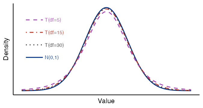
Compared to a t distribution (that approximates a std normal):
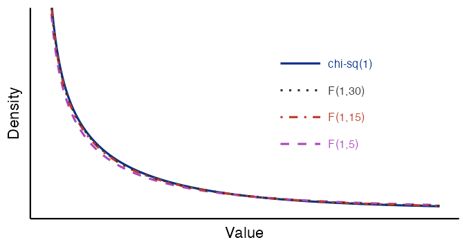
We expect an F distribution (that approximates a \(\chi^2(1)\)):
F-Distribution: Critical Values
Just like our standard normal and T, we can compute inverse probabilities or critical values for our \(F(v_1,v_2)\) distribution with:
Ftail(v1,v2,F)\(\rightarrow P[F>f]\)invFtail(v1,v2,\(\alpha\))\(\rightarrow F^*\text{ s.t. }P[F>F^*]=\alpha\)
A shortcut is that the null of a joint test with \(v_2=n-k>10\) will always be rejected if \(F>5\) for any \(v_1\).
Default F-Test: Overall Significance
Like our default t-tests for \(\beta_j=0\), Stata also runs a default F-test for us: the test of overall significance. This tests whether or not all of our regressors are jointly able to explain variation in our outcome variable: \[H_0: \beta_2=\beta_3=\beta_4=...=0\] \[H_A:\text{ at least one }\beta_j\neq0\]
Note: we do not need all our parameters to be nonzero to reject this null. Instead, we say that at least one of these parameters need be nonzero.
F-Test Output in Stata
We can see Stata compute this default joint F-test of overall significance for us and report the corresponding p-value in our regression output:
      Source |       SS           df       MS      Number of obs   =        69
-------------+----------------------------------   F(3, 65)        =     10.71
       Model |   190778138         3  63592712.8   Prob > F        =    0.0000
    Residual |   386018821        65  5938751.09   R-squared       =    0.3308
-------------+----------------------------------   Adj R-squared   =    0.2999
       Total |   576796959        68  8482308.22   Root MSE        =      2437

------------------------------------------------------------------------------
       price | Coefficient  Std. err.      t    P>|t|     [95% conf. interval]
-------------+----------------------------------------------------------------
         mpg |  -24.44972   85.04044    -0.29   0.775    -194.2872    145.3878
      weight |   2.214518   .6572859     3.37   0.001     .9018274    3.527209
    headroom |  -674.1284   394.8313    -1.71   0.093    -1462.661    114.4041
       _cons |   1974.477   3603.676     0.55   0.586    -5222.561    9171.514
------------------------------------------------------------------------------
Interpreting the F-Test
In this example, we have three coefficients of interest that we set equal to zero (three linear restrictions) in our test of overall significance, \(\beta_2,\beta_3,\beta_4\), so our \(v_1=3\).
We have \(k=4\) total coefficients including our constant term and 69 observations, so our \(v_2=n-k=69-4=65\). For a test of overall significance, our \((v_1,v_2)\) will be (\(k-1,n-k\)).
Thus, Stata reports \(F(3,65)=10.71\) with p-value \(\approx0\). We reject our null hypothesis for the overall significance test and say that at least one regressor does statistically significantly predict our outcome variable (but we cannot say which one).
Unrestricted and Restricted Models
Our F-test operates by comparing what we call the unrestricted model and the restricted model. The unrestricted model is our regression as normal. The restricted model is our original model with all of our linear restrictions added in.
In the case of our overall significance test, we had linear restrictions that the coefficients on all regressors were zero: \(\beta_2=...=\beta_k=0\). Thus, we would plug these into our regression: \[\begin{align*} \text{Unrestricted model: } y &= \beta_1+\beta_2x_2+...+\beta_kx_k+u \\ \text{Restricted model: }y &= \beta_1+0x_2+...+0x_k+u\\ &= \beta_1+u \end{align*}\] We then compare the explanatory power of both models. We reject the null if our unrestricted model explains variation in our outcome variable statistically significantly more than our restricted model.
Computing the F-Statistic
Under assumptions (1)-(4) for our population multivariate regression model, we can compute our F-statistic as:
\[F=\frac{(ResSS_r-ResSS_u)/q}{ResSS_u/(n-k)}\]
where \(ResSS_i\) is the residual sum of squares from our unrestricted (u) and restricted (r) models, respectively, and \(q\) is the number of linear restrictions we make.
For the test of overall significance, \(q=k-1\).
The F-Test is Two-Sided
While our F distribution is right-skewed and bounded below at zero (and thus we are only testing whether \(F>F^*\)), our F-test is still a two-sided test. This should make intuitive sense, as we are testing whether or not one or more linear restrictions between parameters hold. If these assumptions do not hold, it could be in either direction: \(\beta_j<0\) or \(\beta_j>0\).
In the simplest case of testing a single regressor, we saw that \(F_{1,v_2}=(T_{v_2})^2\), further cementing that our F-test is a two-sided test. A positive or negative t-statistic will always become a positive number when squared into an F-statistic: \((-t)^2=F\) and \((t)^2=F\).
Types of F-Tests
We have seen an F-test for overall significance, the test run by default in Stata for any regression. However, we may also have F-tests for:
A subset of regressors, where we compare models with and without a set of linear restrictions. Most commonly this is setting some coefficients equal to zero, but could also be more complicated linear restrictions.
A single regressor, which will give the same p-value as the corresponding t-test on that single regressor.
For all F-tests, our first degrees of freedom measure is the number of linear restrictions we make going from the unrestricted to the restricted model and the second degrees of freedom measure is \(n-k\) as before.
Limiting Distribution: Chi-Squared
We described the standard normal distribution as the limiting distribution of our t distribution: \(T(n-k)\rightarrow N(0,1)\) as \(n\rightarrow\infty\)
Our standard normal distribution always looks the same regardless of sample size. Our t distribution will look more and more like the standard normal (kurtosis\(\rightarrow3\)) as our sample size increases.
The chi-squared \(\chi^2(q)\) distribution is the limiting distribution for our F distribution. A chi-squared distribution is also right-skewed and takes only non-negative values.
Our chi-squared distribution with \(v_1=q\) will also always look the same regardless of sample size. Our F distribution with \(v_1=q\) will look more and more like a scaled chi-squared distribution as our sample size increases: \(q\cdot F(q,n-k)\rightarrow\chi^2(q)\) as \(n\rightarrow\infty\).
End of lecture material
Knowledge Check 11
Consider the Cobb-Douglas model of production: \[Y=AK^{\beta_2}L^{\beta_3}\] We can log transform3 both sides to yield something we can estimate with multivariate OLS: \[\ln Y = \ln A + \beta_2\ln K + \beta_3\ln L\]
Suppose we want to test the assumption of constant returns to scale: that \(\beta_2+\beta_3=1\). Describe and explain how we could conduct this test (and interpret its output) using:
A pooled t-test
An F-test
Knowledge Check 11 — Pooled t-Test Answer
To test our assumption of CRS using a pooled t-test, we would write down the following hypotheses: \[H_0:\beta_2+\beta_3=1\] \[H_A:\beta_2+\beta_3\neq1\] We would then run a log-log regression to estimate: \[\ln Y = \beta_1 + \beta_2\ln K + \beta_3\ln L+u\] with a dataset containing \(Y\), \(K\), and \(L\) and find \(b_2,b_3\) along with standard errors.
Finally, we would conduct a pooled t-test and construct the statistic: \[t=\frac{b_2+b_3-1}{se(b_2
+b_3)}\sim T(n-3)\] where \(se(b_2+b_3)\) is the pooled standard error for \(b_2,b_3\) (that we did not write down in detail). We would then compare this to a critical value \(t^*_{n-3,\alpha/2}\) from invttail().
If \(|t|>|t^*|\), we will reject the null and conclude our economy does not exhibit constant returns to scale. If \(|t|\leq|t^*|\), we will fail to reject the null and conclude our economy does appear to exhibit constant returns to scale. We could also convert our t-statistic into a p-value and compare this to \(\alpha\) to make the same conclusion.
Knowledge Check 11 — F-Test Answer, Part 1
To test our assumption of CRS using a joint F-test, we would write down the following: \[H_0:\beta_2+\beta_3=1\] \[H_A:\beta_2+\beta_3\neq1\]
We would then estimate two regressions — the restricted model (r) and unrestricted model (u). The unrestricted model would be our normal regression: \[\ln Y = \beta_1 + \beta_2\ln K + \beta_3\ln L+u \tag{1}\]
The restricted model would be our regression with the assumptions made under the null plugged into our model. In this case, we could solve for either \(\beta_2\) or \(\beta_3\): \[H_0: \beta_2 = 1-\beta_3\text{ or }\beta_3=1-\beta_2\] Now we can plug this into our unrestricted model to get our restricted model: \[\ln Y = \beta_1 + (1-\beta_3)\ln K + \beta_3\ln L + u \tag{2}\]
Knowledge Check 11 — F-Test Answer, Part 2
Finally, we will estimate models (1) and (2) with OLS and compute the \(ResSS\) for each. We will then construct our F-statistic with: \[F=\frac{(ResSS_r-ResSS_u)/q}{ResSS_u/(n-k)}\sim F(1,n-3)\] where \(q\) is our number of linear restrictions, in this case \(q=1\), \(k\) is our number of estimated regression coefficients, in this case \(k=3\), and \(n\) is our sample size.
We will then compare this F-statistic to a critical value \(F^*_{q,n-k,\alpha}\) we obtain with the invFtail() function in Stata.
If \(F>F^*\), we will reject the null and conclude our economy does not exhibit constant returns to scale. If \(F\leq F^*\), we will fail to reject the null and conclude our economy does appear to exhibit constant returns to scale. We could also convert our F-statistic into a p-value with Ftail() and compare this to \(\alpha\) to make the same conclusion.