ECN 102: Analysis of Economics Data
Chapter 12: Errors and Prediction
Standard Errors: Overview
Our standard error for a statistic is our best estimate for the population standard deviation of that statistic. From this measure, we derive our inference about a population parameter from our sample estimation. Thus, it is critical that we are using the proper standard error for a given setting. We will think about a few cases where typical standard errors would be inappropriate and would lead to improper statistical inference.
Robust Standard Errors
We have discussed the first case already: robust standard errors. Just like in the bivariate case, we invoke robust standard errors (with the robust option in Stata) to address possible threats to homoskedasticity. It is common practice in Economics to default to using robust standard errors, since our assumption of homoskedasticity frequently is violated.
We do not worry about over-using robust standard errors, as these errors are valid even if homoskedasticity does hold. However, if it does not hold, non-robust standard errors would be incorrect. Our use of robust standard errors relaxes our third assumption to be:
\[V[u_i|x_{2i},\dots,x_{ki}]=\sigma^2_{ui},\hspace{5pt} \text{for all }i\]
Clustered Standard Errors
In addition to being heteroskedastic, we may think that our errors are correlated for given sets of observations and thus violate independence. In this case, we would want to cluster our standard errors by some group variable \(G\) to address this threat to the fourth assumption.
For example, if we are studying the effect of a farm subsidy program on household crop outcomes, we may anticipate that harvests would be correlated for all households in a given village due to similar weather conditions. In this case, we would want to cluster our standard errors at the G=village level, to account for the fact that:
Errors within a village may be correlated (not independent)
Errors between villages are not correlated (independent)
Clustered Standard Errors: Modified Assumptions
Clustering our standard errors automatically implements robust standard errors and changes our four population assumptions:
\(2_{clu}\): Cluster unbiasedness \[E[u_i|x_{2i},...x_{ki},x_{2j},\dots,x_{kj}]=0\text{ for }i\text{ and }j\text{ in the same cluster}\]
\(3_{clu}\): Cluster heteroskedasticity (is allowed) \[V[u_i|x_{2i},\dots,x_{ki}]=\sigma^2_{ui}\text{ for all }i\]
\(4_{clu}\): Cluster independence \[Corr[u_i,u_j|x_{2i},\dots,x_{ki},x_{2j},\dots,x_{kj}] \begin{cases} \neq 0 & i\text{ and }j\text{ in the same cluster}\\ = 0 & i\text{ and }j\text{ in different clusters} \end{cases}\]
Bootstrapped Standard Errors
Finally, we may suspect our data does not even fulfill linearity (\(y=\beta_1+\beta_2x_2+...+\beta_kx_k+u\)). In this case, our estimated standard errors for \(b_2,\dots,b_k\) may be incorrect and we need to bootstrap.
Bootstrapping is essentially treating our sample as the population and resampling rows of observations (with replacement) a large number of times to compute new statistics. Then, the variation across our different bootstrap samples gives us a “bootstrapped” estimate of our standard error for that statistic.
The simplest form of bootstrapping we consider here cannot accommodate error clustering but is valid under heteroskedasticity. We could also resample clusters of observations instead of rows to accommodate error dependence within clusters (and possible heteroskedasticity) but generally need at least 30-50 clusters.
Bootstrap: Example Procedure
For example, if we want to bootstrap our standard error of \(b_j\) (without clustering) for a sample \(n=5\) of \((x_2,\dots,x_k,y)\), we would:
Draw \(S\) samples \((x_2,\dots,x_k,y)\) of size \(n=5\) from our “population” of data with replacement
Estimate our \(b_j^*\) for each of these samples and compute the mean across these samples, \(\bar{b_j^*}\)
Compute std. err. \(s_{b_j}^{boot}=\sqrt{\frac{1}{S-1}\sum_{s=1}^S\left(b_{j_s}^*-\bar{b_j^*}\right)^2}\)
Compare this estimate to the OLS standard error \(s_{b_j}\)
If our population model was nonlinear, we would expect to find \(s_{b_j}^{boot}\neq s_{b_j}\) indicating our regular OLS standard errors were misestimating the variability of \(b_j\) due to our model being ill-fitting. We should therefore adjust our regression.
Choosing the Right Standard Error
Do you suspect…
Heteroskedasticity? \(\Rightarrow\) robust standard errors
reg y x, robustError dependence within clusters? \(\Rightarrow\) clustered standard errors
reg y x, vce(cluster G)Non-linearity? \(\Rightarrow\) bootstrapped standard errors
bootstrap, reps(S): reg y xNon-linearity AND error dependence within clusters? \(\Rightarrow\) clustered bootstrapped standard errors
bootstrap, reps(S) cluster(G): reg y x
Prediction: Average vs. Individual Values
We may want to use our regression to predict both average values and individual values of our outcome based on our regressors. Average values will be the conditional mean of y, \(E[y|x_2,\dots,x_k]\), while actual values will be the conditional value of y, \(y|x_2,\dots,x_k\). It should be clear that the second quantity will be more widely dispersed than the first; it represents the full range of outcome values we might expect, not just the average values in the middle.
In both cases, we would use \(y|x^*_2,\dots,x_k^*\) for a given \(x=x^*\) by multiplying our regressor values by our estimated coefficients, but we would also need to consider the variance of the error term \(u\) for our individual values. We do not know very much about this error (besides it being conditional mean zero under assumption 2) but it will affect how spread out our predicted individual values will be.
Power: Definition
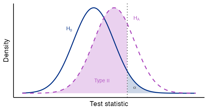
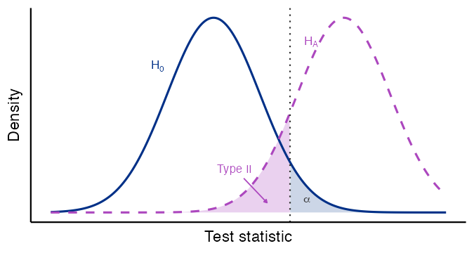
Previously, we defined our test size as the \(P[\text{Type I}]=\alpha\) but left a discussion of our Type II error probability ambiguous. Now, we can more precisely define the power of our test as \(1-P[\text{Type II}]\), which we seek to maximize for a given test size.
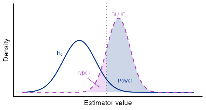
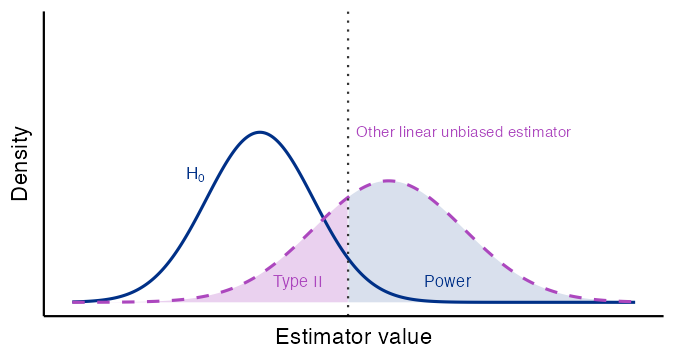
If we are able to choose our sample size, we may need to calculate an \(n\) such that our results will be well-powered: our standard errors will not be enormous and our results will be believable. Of course, it is often very expensive to increase our sample size, so we balance constraints on sampling with concerns about power. As before, we further cement the power of our tests by using our best estimators, or those with minimum variance in their class, to reduce the chances of a Type II error as much as possible.
Type I vs. Type II Errors
Whether our decision to reject or fail to reject \(H_0\) (from the sample) is correct depends on the truth (in the population). The two ways we can be wrong are the Type I error and the Type II error:
| True state of the world | |||
|---|---|---|---|
| θ = θ0 | θ ≠ θ0 | ||
| Decision | Reject H0 | Type I error (α) | Correct — power (1−β) |
| Fail to reject H0 | Correct (1−α) | Type II error (β) | |
A Type I error is a false positive (rejecting a true \(H_0\)); a Type II error is a false negative (failing to reject a false \(H_0\)).
Power: Type II Error Regions
Large type II error region:
Small type II error region:
Power: Estimator Distribution
Parameter assumption and “best estimator” distribution:
Parameter assumption and other estimator distribution:
Multiple Hypothesis Testing
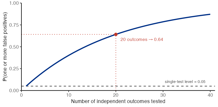
For a single test, we know that \(P[\text{Type I}]=\alpha\). If we run many tests (each at the 5% level), this becomes a serious problem: with 20 independent true nulls, the chance of at least one false positive is \(1 - (1 - 0.05)^{20} \approx 0.64\). Although we will not dig into the methodology in this class, we should consider additional measures to employ when we are doing many individual tests on the same sample of data to account for the fact that some of our results may be false positives. We call these multiple hypothesis corrections.
We also want to avoid p-hacking: running many tests but only reporting those where we find significance. This again compounds our Type I error probability and invalidates our inference.
Testing Many Outcomes: False Positives Multiply
End of lecture material
Knowledge Check 12
Consider a test for some parameter \(\theta\) (e.g. \(\beta_2\)) with: \[H_0:\theta=0\] \[H_A:\theta\neq0\]
Suppose we know that the probability of rejecting \(H_0\) is 0.10 when \(\theta=0\) and 0.75 when \(\theta\neq0\). Please give:
The size of the test
The probability of a type I error
The probability of a type II error
The power of the test
Suppose \(n\) is fixed. What could we do to ensure our test is as well-powered as possible?