      Source |       SS           df       MS      Number of obs   =        74
-------------+----------------------------------   F(3, 70)        =      9.48
       Model |   183435281         3  61145093.6   Prob > F        =    0.0000
    Residual |   451630115        70  6451858.79   R-squared       =    0.2888
-------------+----------------------------------   Adj R-squared   =    0.2584
       Total |   635065396        73  8699525.97   Root MSE        =    2540.1

------------------------------------------------------------------------------
       price | Coefficient  Std. err.      t    P>|t|     [95% conf. interval]
-------------+----------------------------------------------------------------
         mpg |  -329.2551   74.98545    -4.39   0.000    -478.8088   -179.7013
     foreign |  -13.58741   2634.664    -0.01   0.996    -5268.258    5241.084
 mpgXforeign |   78.88826   112.4812     0.70   0.485    -145.4485     303.225
       _cons |   12600.54   1527.888     8.25   0.000     9553.261    15647.81
------------------------------------------------------------------------------ECN 102: Analysis of Economics Data
Chapter 14: Indicator Variables
Remy Beauregard
Canvas Announcement: Final Exam Review Session
I will be holding extra office hours on Tuesday morning 10am-12pm before class in SSH 136 as a chance to ask any questions about class material.
I will also be holding an exam review session Tuesday afternoon 3-5pm after class in the Gold Room (SSH 1131) to go over additional practice questions for the exam (that will also be posted on our website). This will be another chance to ask any questions about class material.
I realize we are covering two new chapters the week of the exam and want to ensure sufficient time to digest and understand the material. The review session will thus be focused mostly on material from later chapters. While these are not mandatory, I highly recommend attending as you prepare for the final exam.
Indicator Variables: Introduction
We previously asserted that categorical variables, such as shirt color, are not typically included in regression, since it is difficult to interpret a numerical coefficient for a discrete categorical series.
One common exception is using indicator variables which encode categorical information. A special kind of indicator variable is called a dummy variable which is coded as being only zero or one.
We may have a single indicator variable for a binary outcome (male=1 vs. male=0) or a set of indicator variables that span the possible options (red shirt, blue shirt, green shirt, …). Indicator variables give us a powerful way to analyze differences in means and slopes for different groups within our regression.
Simple Dummy Variable Regression
Suppose we want to estimate the average final grade in ECN102 for Econ majors and non-majors. We could define a dummy variable \(ECN=1\) for Economics majors and 0 otherwise.
We then estimate \(final_i=\beta_1+\alpha_1 ECN_i+u_i\):
\[\widehat{final}_i=\begin{cases} b_1+a_1 & ECN_i =1 \\ b_1 & ECN_i=0 \end{cases}\]
Our coefficient \(a_1\) on \(ECN\) is then the average difference in final grade between Econ majors and non-majors. This is the simplest use of a dummy variable.
Graph: Final Grade on ECN Major Status
\(\widehat{final}_i=b_1+a_1 ECN_i\):
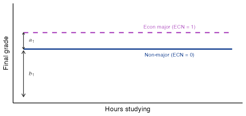
Schematic regression lines showing the effect of a binary dummy variable on the outcome, with no continuous regressor.
Dummy Variables in Multivariate Regression
We may also want to include dummy variables in a multivariate regression with other continuous numerical regressors. In this case, the partial effect (estimated coefficient) of the dummy variable is the change in our outcome when our dummy goes from 0 to 1, all other regressors held constant. The total effect is our partial effect added to the product of any correlated movement in other variables and its associated coefficient.
We now estimate: \[final_i=\beta_1+\beta_2hrs_i+\alpha_1 ECN_i+u_i\] where \(hrs\) is the number of hours spent studying and \(ECN=1\) is being an Econ major. Now, our estimated coefficient \(a_1\) is the average difference in final grades between Econ majors and non-majors holding time spent studying fixed.
Graph: Final Grade, Hours, and ECN Major Status
\(\widehat{final}_i=b_1+b_2hrs_i+a_1 ECN_i\):
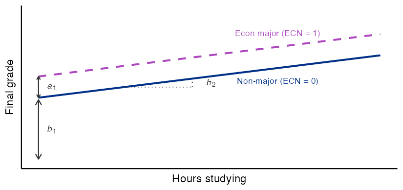
Schematic parallel regression lines showing a binary dummy variable added to a regression with a continuous regressor.
Interacting a Dummy Variable with a Regressor
Finally, we could interact our dummy variable with another regressor to capture the average difference in slopes between one category and another. Adding to our regression of final grades, we could estimate: \[final_i=\beta_1+\beta_2hrs_i+\alpha_1ECN_i+\alpha_2(ECN_i\times hrs_i)+u_i\]
\(\beta_2\) captures the change in final grade associated with 1 additional hour of studying for non-majors
\(\alpha_1\) captures the average difference in overall final grades between majors and non-majors
\(\beta_2+\alpha_2\) captures the change in final grade associated with 1 additional hour of studying for majors
Graph: Interacted Dummy Regression
\(\widehat{final}_i=b_1+b_2hrs_i+a_1ECN_i+a_2(ECN_i\times hrs_i)\):
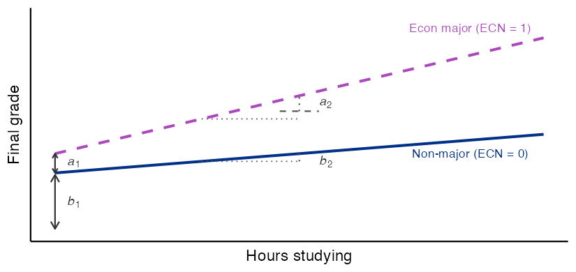
Schematic regression lines showing a binary dummy variable interacted with a continuous regressor.
Interpreting the Interacted Dummy: Slopes and Intercepts
For an interacted dummy variable regression: \[\hat{y}_i=b_1+b_2x_i+a_1d_i+a_2(d_i\times x_i)\]
\(a_1>0\) means the intercept for \(d=1\) is higher than for \(d=0\)
\(a_1<0\) means the intercept for \(d=1\) is lower than for \(d=0\)
\(a_2>0\) means the slope for \(d=1\) is steeper than for \(d=0\)
\(a_2<0\) means the slope for \(d=1\) is less steep than for \(d=0\)
If \(a_2\) is larger than \(b_2\) in magnitude but has the opposite sign, the slope for \(d=1\) will go in the opposite direction from that for \(d=0\).
Interacted Dummy: Two Separate Group Regressions
Plugging in \(d=0\) and \(d=1\), we see that we are actually just running two different bivariate regressions for two groups: \[\begin{aligned} d_i=0\text{: }\hat{y}_i&=b_1+b_2x_i+a_1d_i+a_2(d_i\cdot x_i)\\ &=b_1+b_2x_i+a_1(0)+a_2(0)x_i\\ &=b_1+b_2x_i \end{aligned}\] \[\begin{aligned} d_i=1\text{: }\hat{y}_i&=b_1+b_2x_i+a_1d_i+a_2(d_i\cdot x_i)\\ &=b_1+b_2x_i+a_1(1)+a_2(1)x_i\\ &=b_1+b_2x_i+a_1+a_2x_i\\ &= \underbrace{(a_1+b_1)}_{c_1} + \underbrace{(a_2+b_2)}_{c_2}x_i\\ &=c_1+c_2x_i \end{aligned}\]
Interacted Dummy: Standard Errors of Linear Combinations
From the preceding derivation, the interacted regression estimates \(b_1+b_2x_i\) for \(d_i=0\) and \((a_1+b_1)+(a_2+b_2)x_i\) for \(d_i=1\).
Point estimate: The total slope for \(d=1\) is \(c_2=a_2+b_2\), obtained directly by adding the two estimated coefficients from the regression table.
Standard error: Computing \(\text{se}(c_2)\) is more involved. Because \(c_2\) is a linear combination of two estimates, its variance depends on both individual variances and their covariance:
\[\text{se}(c_2)=\sqrt{V[a_2]+V[b_2]+2\,\text{Cov}[a_2,b_2]}\]
We compute both in Stata using the lincom command.
Example: Car Prices, MPG, and Country of Origin
How would we interpret the following regression results with indicator variable foreign?
\[\text{Pop. model: }price_i=\beta_1+\beta_2mpg_i+\alpha_1foreign_i+\alpha_2(mpg_i\times foreign_i)+u_i\] \[b_1=12600.54\] \[b_2=-329.26\] \[a_1=-13.59\] \[a_2=78.89\]
Graph: Price on MPG by Country of Origin
Graph of \(price\) on \(mpg\) across \(foreign\):
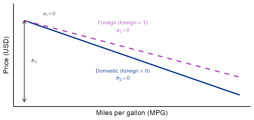
Schematic regression lines for price on MPG by country of origin.
Ordered and Unordered Categorical Variables
We may use indicator variables that take values other than 0 or 1 if we have an ordered or ranked categorical variable, such as class year (freshman, sophomore, etc.). We could capture these with a single variable called \(Class\) which takes values 0, 1, 2, or 3 depending on the incoming year (with 4 for super-senior+). Our only caveat in this case would be that we are assuming the effect of going from freshman to sophomore is the same as going from junior to senior.
For unordered categorical variables, we may instead want to use a set of dummy variables, each representing a category in our set, such as shirt colors. We say these dummies are mutually exclusive and exhaustive if all observations fall into exactly one category. We can check this by summing the sample means for our dummies — they should sum to 1 exactly.
The Dummy Variable Trap
We previously discussed the issue of perfect collinearity between regressors — we cannot estimate two separate regressors that are exact linear combinations of each other. For dummy variables, this means we cannot include dummy variables for all categories in our regression without errors — we must leave out one variable. We call this group, unsurprisingly, the leave-out group, and all regression results are compared to this group. We may want to choose this group carefully to yield the best interpretation of our results.
Failing to remove one mutually exclusive dummy variable from a set that spans all categories is called the dummy variable trap and will lead to errors in estimation. We can also avoid this by including all dummies but dropping the constant term.
Why the Dummy Variable Trap Occurs
Why do we encounter the dummy variable trap?
Suppose we have a category \(c\) that takes values 1, 2, or 3 and every observation falls into exactly one category. Now suppose we construct dummy variables \(d_1,d_2,d_3\) for if an observation falls into category 1, 2, or 3, respectively.
If \(d_1=0\) and \(d_2=0\), it must be the case that \(d_3=1\).1
We can then rewrite \(d_3\) as \(d_3=1-d_1-d_2\). This means \(d_3\) is a linear combination of other regressors in our model and thus perfectly collinear. If we try to include \(d_3\) in our model along with \(d_1\) and \(d_2\), we will not be able to estimate our coefficients.
Rule: At Most n−1 Dummy Variables
Generally, if we have \(n\) mutually exclusive and exhaustive categories each with a dummy variable, we can include at most \(n-1\) dummy variables in our regression (\(d_1,...,d_{n-1}\)).
The last dummy variable, \(d_n\), would be equal to: \[d_n=1-\sum_{i=1}^{n-1}d_i\]
More generally, if we choose the dummy variable for category \(j\) to be our leave-out group, we will include all dummies \(d_{i\neq j}\) in our regression and have \(d_j=1-\sum_{i\neq j}d_i\).
Inference on Dummy Variables
When we conduct inference on dummy variables with a leave-out group, we are not testing whether the included dummy is different from zero, but rather if the difference between that group and the leave-out group is zero. Our F-test for overall significance, however, still measures whether all included regressors meaningfully predict our outcome variable.
Example: Values of the Foreign Variable
In our car example, we can find the unique values of our categorical variable foreign using frequency foreign:
foreign -- Car origin
----------------------------------------------------------------
                   |      Freq.    Percent      Valid       Cum.
-------------------+--------------------------------------------
Valid   0 Domestic |         52      70.27      70.27      70.27
        1 Foreign  |         22      29.73      29.73     100.00
        Total      |         74     100.00     100.00
----------------------------------------------------------------
To estimate a regression using dummies for foreign, we would need to either:
Include only a dummy on foreign and not domestic
Include only a dummy on domestic and not foreign
Drop our constant term and include both dummies
Avoiding the Dummy Variable Trap
Do we run into the dummy variable trap here? Why or why not?
      Source |       SS           df       MS      Number of obs   =        74
-------------+----------------------------------   F(3, 71)        =    155.75
       Model |  2.9930e+09         3   997676875   Prob > F        =    0.0000
    Residual |   454803695        71  6405685.84   R-squared       =    0.8681
-------------+----------------------------------   Adj R-squared   =    0.8625
       Total |  3.4478e+09        74  46592355.7   Root MSE        =    2530.9

------------------------------------------------------------------------------
       price | Coefficient  Std. err.      t    P>|t|     [95% conf. interval]
-------------+----------------------------------------------------------------
         mpg |  -294.1955   55.69172    -5.28   0.000    -405.2417   -183.1494
    domestic |   11905.42   1158.634    10.28   0.000     9595.164    14215.67
     foreign |   13672.71   1481.406     9.23   0.000     10718.87    16626.55
------------------------------------------------------------------------------
\[\widehat{price}_i=b_2mpg_i+\delta_1domestic_i+\delta_2foreign_i\]
Creating Factor Variable Dummies in Stata
We can easily create dummies for these discrete mutually exclusive factor variables in Stata:
We can also call on dummy variables directly in our regression. However, Stata makes us first convert categorical variables into numeric variables before we do this (R does not):
End of Lecture Material
Knowledge Check 14
Suppose we estimate the following regression: \[y_i = \beta_1 + \beta_2x_i + \alpha_1d_i + \alpha_2(d_i\times x_i)+ u_i\] where \(d\) is a dummy variable for being in category \(C\) or not. How would we interpret the coefficients \(b_1,b_2,a_1,\) and \(a_2\)?