Contains data from HEALTH2009.dta
 Observations:            34                  Data for A. Colin Cameron
                                                (2022), ANALYSIS OF ECONOMIC
                                                DATA, Amazon
    Variables:            13                  22 Jan 2022 14:34
-------------------------------------------------------------------------------
Variable      Storage   Display    Value
    name         type    format    label      Variable label
-------------------------------------------------------------------------------
country_name    str15   %15s                  Country name, OECD
year            int     %9.0g                 Year
hlthgdp         float   %8.0g                 Health as % of GDP
hlthpc          int     %8.0g                 Health expenditure per capita
infmort         float   %8.0g                 Infant Mortatility (deaths per
                                                1,000)
lifeexp         float   %8.0g                 Male Life Expectancy (years)
gdppc           float   %8.0g                 GDP per capita
code            str3    %9s                   Three letter country code
hlthpcsq        float   %9.0g                 Health expenditure per capita
                                                squared
lnhlthpc        float   %9.0g                 Natural logarithm of hlthpc
lngdppc         float   %9.0g                 Natural logarithm of GDP per
                                                capita
lnlifeexp       float   %9.0g                 Natural logarithm of Life
                                                expectancy
lninfmort       float   %9.0g                 Natural logarithm of Infant
                                                mortality
-------------------------------------------------------------------------------
Sorted by: country_name yearECN 102: Analysis of Economics Data
Chapter 8: Bivariate Practice (With Answers)
Dataset Overview
- What would be some sensible explanatory variables? Some outcome variables?
hlthgdp, hlthpc, gdppc might be some sensible independent variables; infmort, lifeexp might be some sensible dependent variables.
Health Spending Distribution
                     Health as % of GDP
-------------------------------------------------------------
      Percentiles      Smallest
 1%          6.4            6.4
 5%          6.7            6.7
10%            7            6.9       Obs                  34
25%            8              7       Sum of wgt.          34

50%          9.6                      Mean           9.673529
                        Largest       Std. dev.      2.123934
75%         10.8           11.7
90%         11.7           11.7       Variance       4.511096
95%         11.9           11.9       Skewness       1.364484
99% 17.7 17.7 Kurtosis 7.107991- How would we describe this variable in words? What are its measures of central tendency? Spread? What do these each mean?
Our variable has a mean of 9.67 with a median of 9.6, indicating a right-skew. We confirm this with a skewness \(>0\). We have thicker tails than a normal distribution with \(Kurt>3\). Our standard deviation is 2.12. Our IQR is 10.8-8=2.8.
Infant Mortality and Life Expectancy
    Variable |        Obs        Mean    Std. dev.       Min        Max
-------------+---------------------------------------------------------
     infmort |         34    4.447059    2.720098        1.8       14.7
lifeexp | 34 76.70294 2.936756 69.8 79.9- Which of these two variables has greater spread relative to its mean? How do we know?
\[CV=\frac{s}{\bar{x}}: \frac{2.72}{4.45} > \frac{2.94}{76.70}\Rightarrow\text{infmort has larger dispersion}\]
- What would we expect the standard error (of \(\bar{x}\)) of infmort to be?
\[se(\overline{infmort})=\frac{s_{\text{infmort}}}{\sqrt{n}}=\frac{2.72}{\sqrt{34}}\]
Regression of Life Expectancy on Health Spending
Suppose we regress lifeexp on hlthgdp:
      Source |       SS           df       MS      Number of obs   =        34
-------------+----------------------------------   F(1, 32)        =      6.62
       Model |  48.7766651         1  48.7766651   Prob > F        =    0.0149
    Residual |   235.83297        32   7.3697803   R-squared       =    0.1714
-------------+----------------------------------   Adj R-squared   =    0.1455
       Total |  284.609635        33  8.62453438   Root MSE        =    2.7147

------------------------------------------------------------------------------
     lifeexp | Coefficient  Std. err.      t    P>|t|     [95% conf. interval]
-------------+----------------------------------------------------------------
     hlthgdp |   .5724111   .2224996     2.57   0.015     .1191942    1.025628
       _cons |   71.16571   2.202135    32.32   0.000     66.68011    75.65131
------------------------------------------------------------------------------
Population Model and OLS Assumptions
Population model:
- What is the population model we are estimating?
\[\text{lifeexp}_i = \beta_1 + \beta_2 \text{hlthgdp}_i + u_i\]
- What four assumptions do we make to use OLS?
- Linearity, (2) Unbiasedness, (3) Homoskedasticity, (4) Independence
- What would be a potential threat to each assumption?
Nonlinear relationship between X and Y
An omitted variable in our regression
Heteroskedasticity - non-uniform distribution of errors
Correlation in our errors between observations
Sample Estimates
Sample estimate:
- What is \(b_1\)? What is \(b_2\)? What are these in words? What do these estimate?
\(b_1=71.166\) is our intercept; \(b_2=0.572\) is our slope. We expect a country that spends 0% of its GDP on health to have a male life expectancy of around 71 years and to gain roughly half a year of life expectancy for each 1% additional of GDP spent on health. These estimate \(\beta_1\) and \(\beta_2\) from the population model.
- What are some properties of our estimator \(b_2\)?
We know our OLS estimator to be unbiased \((E[b_2]=\beta_2)\), consistent \((\sigma^2_{b_2}\rightarrow0\text{ as }n\rightarrow\infty)\), and BLUE (Best Linear Unbiased Estimator) with minimum variance of all similar estimators.
More Sample Estimates
- What is \(s_{b_2}\)? How is this different from \(\sigma_{b_2}\)?
\(s_{b_2}\) is the standard error for our slope coefficient, calculated using all sample quantities. This is our sample estimate of precision for \(b_2\). Our population standard deviation for \(b_2\), \(\sigma_{b_2}\), would use population parameters instead (\(\sigma_u\) instead of \(s_e\)) and is the population standard deviation of our slope coefficient.
- What would we expect the male life expectancy to be for a country that spends 7% of its GDP on health?
\(E[Y|X=7]=71.166+0.572\times7=75.17\)
Model Fit
Model fit:
- What is our ExpSS? Our ResSS? Our TSS?
\(ExpSS=48.78;\ ResSS=235.83;\ TSS=284.61\)
- What is our \(R^2\)? What is \(r_{xy}\)? What do these each mean?
\(R^2=0.1714;\ r_{xy}=\sqrt{0.1714}=0.41\). 17.14% of our variation in male life expectancy is explained by (variation in) health spending as a % of GDP. The two variables have a moderate positive correlation of 0.41 (remember the sign of \(r_{xy}\) is the same as the sign of \(b_2\)).
More Model Fit
- Can we say \(b_2=r_{xy}\)? Why or why not?
We cannot say \(b_2=r_{xy}\) without knowing \(s_x\) and \(s_y\), since we know \(b_2=r_{xy}\frac{s_y}{s_x}\). It is unlikely the two are exactly equal.
- What are two ways we could calculate \(R^2\) manually?
\(R^2 = \frac{ExpSS}{TSS}=1-\frac{ResSS}{TSS}=\frac{48.78}{284.61}=1-\frac{235.83}{284.61}=0.1714\)
Bivariate Inference
Bivariate inference:
- Which hypotheses does the t-statistic for \(b_2\) correspond to?
\(H_0:\beta_2=0\)
\(H_A:\beta_2\neq0\)
- Can we reject this null hypothesis using the p-value approach?
Yes; P>|t| (the probability of getting a test statistic at least as large if the null hypothesis is true) \(=0.015<\alpha=0.05\) so we reject the null. There is a statistically significant association between x and y.
- Can we reject this null using our confidence interval?
Yes; our parameter value assumed under the null is not included in our confidence interval, so we can reject the null. There is a statistically significant association between x and y.
Critical Value and Degrees of Freedom
- Without using
invttail(), what do we know about \(t^*_{df,\alpha/2}\), our critical value?
Since our p-value and critical value approaches must always give us the same answer for whether to reject a given null, we know that \(t=2.57>t^*_{df,\alpha/2}\) even if we do not know \(t^*_{df,\alpha/2}\) itself.
- How many degrees of freedom will our t-statistic above have? Why?
Our test will have \(n-2\) degrees of freedom, because two (2) precomputed quantities are used to calculate our test statistic: \(b_1\) and \(b_2\).
- State the conclusion of our hypothesis test in words.
We reject the null and state that there is a statistically significant association between % of GDP spent on health and male life expectancy.
Scatter Plot
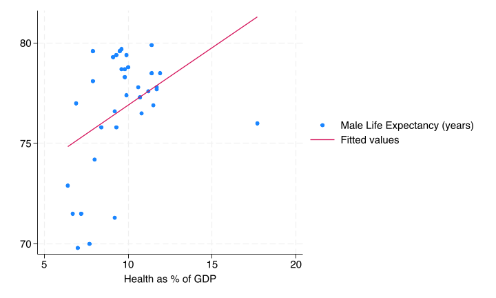
- What do we notice about this regression and data?
Our data is likely both heteroskedastic (more spread at lower values of x) and has an outlier. We may want to drop the outlier and use robust SEs in our regression.
Homoskedasticity and Outlier Discussion
- Which assumption are we now worried our data might violate?
We may be worried our data violates homoskedasticity, our third (3rd) assumption. Our errors appear to be larger for smaller values of x.
- What could we do in response to this concern?
We would need to add the option ,robust to our regression in Stata.
- What quantity(ies) would be changed as a result of this?
Our coefficient estimates would not change as a result of using robust, but our standard errors would change. T-statistics, p-values, and CIs would also change.
- How would our regression change if we instead excluded the right-most point?
Our right-most point is significantly below our regression line, indicating it is likely making our \(b_2\) much lower than it would be without this point.
Ordinary Least Squares: BLUE
- What does our OLS estimator \(b_2\) minimize? What does it maximize?
Our OLS estimator \(b_2\) minimizes the sum of squared residuals, \(\sum_{i=1}^ne_i^2\). By definition, it then also maximizes our coefficient of determination, \(R^2\).
- We called the OLS estimator BLUE - what did this mean?
This means that our OLS estimator is the Best Linear Unbiased Estimator. This means it is (1) unbiased, (2) linear in form, and (3) has minimum variance of all similar estimators. We said (3) was important to minimize Type II error probability.
- Suppose I obtain a sample of data (\(n=63\)) I am certain is not normally distributed. I want to use OLS and conduct inference on \(b_2\), but will I be able to? Why or why not?
The power of the central limit theorem (CLT) says that a statistic computed from a sample with \(n>30\) will be approximately normally distributed, even if the sample data itself is not normally distributed. The \(b_2\) we compute from this data can be expected to follow an asymptotically normal distribution in this case.