Contains data from /Applications/Stata/ado/base/a/auto.dta
 Observations:            74                  1978 automobile data
    Variables:            12                  13 Apr 2022 17:45
                                              (_dta has notes)
-------------------------------------------------------------------------------
Variable      Storage   Display    Value
    name         type    format    label      Variable label
-------------------------------------------------------------------------------
make            str18   %-18s                 Make and model
price           int     %8.0gc                Price ($)
mpg             int     %8.0g                 Mileage (mpg)
rep78           int     %8.0g                 Repair record 1978
headroom        float   %6.1f                 Headroom (in.)
trunk           int     %8.0g                 Trunk space (cu. ft.)
weight          int     %8.0gc                Weight (lbs.)
length          int     %8.0g                 Length (in.)
turn            int     %8.0g                 Turn circle (ft.)
displacement    int     %8.0g                 Displacement (cu. in.)
gear_ratio      float   %6.2f                 Gear ratio
foreign         byte    %8.0g      origin     Car origin
-------------------------------------------------------------------------------
Sorted by: foreign
Note: Dataset has changed since last saved.ECN 102: Analysis of Economics Data
Final Exam SS1 2025 – Answer Key
This exam consists of 5 short-answer questions (with sub-parts) and 5 multiple choice questions. You will have a maximum of 100 minutes to complete this exam. No additional time may be taken without prior accommodation. Show all work to receive full credit. You may use only the calculators provided by the instructor. For questions requiring computation, it suffices to express your final answer with 2 decimal places. There is a formula sheet and scratch paper provided at the end of this exam. You may remove these pages and discard them after the exam. If you plan to use any of these extra pages for your final answers, please write your name and student ID at the top of each to ensure they are not lost.
This exam is worth 100 points.
Question 1: Ordinary Least Squares (OLS) Estimator [15 points]
Suppose we run a multivariate regression of an outcome \(y\) on \(k-1>1\) regressors and a constant for a sample of size \(n\). We will refer to our general OLS estimator as \(b_j\), with \(j=2,...,k\) (we do not care about the constant term but still need to estimate it). Please answer the following:
- What does \(b_j\) represent in words? Please be as specific as possible. [2 points]
\(b_j\) is the associated change in \(y\) when \(x_j\) changes by one unit, all else held constant.
- What is the difference between \(x_j\) and \(\tilde{x}_j\)? [2 points]
\(x_j\) is the total variation of our regressor; \(\tilde{x}_j\) is the unique or independent variation of \(x_j\) not explained/predicted by all other regressors in our model.
- What does it mean for our estimator \(b_j\) to be unbiased? Explain in words. [3 points]
The population mean of the distribution of our estimator is centered at the correct population parameter value; \(\mathbb{E}[b_j]=\beta_j\)
- What does it mean for our estimator \(b_j\) to be consistent? Explain in words. [3 points]
The precision of our estimator \(b_j\) (or variance of the distribution of our estimator) decreases as our sample size grows larger; \(\sigma^2_{b_j}\rightarrow0\) as \(n\rightarrow\infty\).
- What does it mean for our estimator \(b_j\) to be the Best Linear Unbiased Estimator (BLUE)? Explain in words. [3 points]
\(b_j\) is our Best Linear Unbiased Estimator (BLUE), meaning it has the smallest variance of all similar estimators. This means that using \(b_j\) from OLS will maximize the power of our inference relative to any other linear, unbiased estimator.
- If we know our regressor \(x_j\) is not normally distributed, should we still expect \(\beta_j\) to be normally distributed? Why or why not? [2 points]
Yes. The CLT says that we can expect the distribution of a statistic like \(b_j\) to be normally distributed, for a large enough sample, even if the underlying variable(s) are not normally distributed. In order to use OLS, we are assuming that our sample size is large enough to use the CLT.
Question 2: OLS Regression Output [20 points]
We will work with the 1978 automotive dataset. Variables in the dataset and their labels are given below:
Suppose we now estimate a regression model and obtain the following results:
      Source |       SS           df       MS      Number of obs   =        74
-------------+----------------------------------   F(3, 70)        =     11.09
       Model |   204556469         3  68185489.6   Prob > F        =    0.0000
    Residual |   430508927        70  6150127.53   R-squared       =    0.3221
-------------+----------------------------------   Adj R-squared   =    0.2931
       Total |   635065396        73  8699525.97   Root MSE        =    2479.9

------------------------------------------------------------------------------
       price | Coefficient  Std. err.      t    P>|t|     [95% conf. interval]
-------------+----------------------------------------------------------------
         mpg |  -56.19416   85.07654    -0.66   0.511     -225.874    113.4856
      weight |   2.061945   .6586383     3.13   0.003      .748332    3.375557
    headroom |  -675.5962   392.3504    -1.72   0.090    -1458.115     106.922
       _cons |   3158.306   3617.449     0.87   0.386    -4056.468    10373.08
------------------------------------------------------------------------------- Write down the population regression model we are estimating using variable names. [2 points]
\[\boldsymbol{price=\beta_1+\beta_2mpg+\beta_3weight+\beta_4headroom+u}\]
- Write down the sample regression model we have estimated above using variable names. [2 points]
\[\boldsymbol{\widehat{price}=3158.31-56.19mpg+2.06weight-675.60headroom}\]
- Interpret the coefficient on mpg in words. [3 points]
A one unit increase in mpg is associated with a $56.19 lower car price, all else held constant.
- We see the 95% confidence interval for headroom includes zero and that
P>|t|for headroom \(=0.090\). Do these results surprise you? Why or why not? [3 points]
No, these results are not surprising. We know that failing to reject the null of the test of association (\(0.090>\alpha=0.05\)) means the value assumed under the null must fall inside the corresponding 95% confidence interval. As we fail to reject the null, our null value of 0 is also within the interval.
- Interpret the p-value for weight. What null and alternate hypotheses does this p-value correspond to? What is the name of this test? State your full conclusion in words for this test. [4 points]
\(H_0:\beta_3=0\)
\(H_A:\beta_3\neq0\)
\(p=0.003\); this is the probability of drawing a t-statistic at least as large as 3.13 from a \(T(70-4)\) distribution assuming the null is true (assuming there is no statistically significant association between weight and price). We reject the null of the test of association for weight and price and say there is a statistically significant association of weight on price, all else held constant.
- Interpret the \(R^2\) of our regression in words. [2 points]
\(R^2=0.3221\), meaning 32.21% of the variation in price can be accounted for/explained by our model (all regressors together).
- Interpret
Prob>Ffrom the table. What null and alternate hypotheses does this p-value correspond to? What is the name of this test? State your full conclusion in words for this test. [4 points]
\(H_0:\beta_2=\beta_3=\beta_4=0\)
\(H_A:\text{at least one }\beta_j\neq0\)
\(p\approx0\); this is the probability of drawing an F-statistic at least as large as 11.09 from a \(F(3,70-4)\) distribution assuming the null is true (assuming none of our regressors have any power to explain variation in our outcome variable). We reject the null of the test of overall significance and say that at least one of our regressors does statistically explain variation in price, although we cannot say definitively which one(s).
Question 3: Intuition for Inference [16 points]
Here we will ask questions about regression inference (bivariate or multivariate).
- If we write down \(\alpha=0.05\) for a test of inference, what could this quantity represent? [2 points]
(Hint: You should have two answers)
This quantity could represent our statistical significance value, which we compare to our p-value, or to the test size, the probability of committing a Type I error.
- Given our answer above, why would we not want to set \(\alpha=0\)? Why would we not want to set \(\alpha=1\)? Please give a short explanation for each. [4 points]
Setting \(\alpha=0\) would mean never rejecting the null hypothesis; setting \(\alpha=1\) would mean always rejecting the null hypothesis. We would like to be able to reject the null when it is false (\(\alpha>0\)) but also not reject the null when it is true (\(\alpha<1\)). We would like to select \(\alpha\) to balance the chances of a Type I and Type II error.
- Given our standard choice of \(\alpha=0.05\), what are three ways we can maximize the power of our inference? Please give a short explanation for each. [6 points]
To maximize power, we can:
1. Choose to use our best estimator with minimum variance
2. Select the largest sample size possible
3. Target a large rather than small effect size so that our null and alternate distributions are (hypothetically) centered further away from each other.
Suppose we have a test of association for our regression coefficient \(\beta_j\) with standard null and alternate hypotheses. For this test:
- What would it mean to commit a Type I error? [2 points]
This would mean we are rejecting the null when the null is in fact true; there is no statistically significant association between \(x_j\) and \(y\) but we are claiming there is.
- What would it mean to commit a Type II error? [2 points]
This would mean we are failing to reject the null when the null is in fact false; there is a statistically significant association between \(x_j\) and \(y\) but we are claiming there is not.
Question 4: Errors and Prediction [14 points]
Suppose we are worried our data violates homoskedasticity and so choose to use robust standard errors:
- Will this cause our standard errors to grow, shrink, or stay the same size (compared to using default standard errors)? You do not need to explain. [2 points]
Implementing robust standard errors for heteroskedastic data would cause our standard errors to grow compared to the default.
- Will this cause our t-statistics to grow, shrink, or stay the same size (compared to using default standard errors)? Please explain. [3 points]
As we use the standard error in the denominator of our t-statistics, larger standard errors would cause our t-statistics to shrink compared to the default.
- Will this cause our regression coefficients to grow, shrink, or stay the same size (compared to using default standard errors)? Please explain. [3 points]
Using robust standard errors does not affect our coefficient estimates, so these would remain the same.
- Will this cause our confidence intervals to get wider, narrower, or stay the same size (compared to using default standard errors)? Please explain. [3 points]
As we use the standard error to construct our CI, larger standard errors would lead to a wider confidence interval compared to the default.
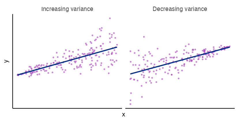
- Suppose we run
scatter y xand confirm our data indeed looks heteroskedastic. Please draw an example of what this scatterplot might look like below. [3 points]
Question 5: OLS and Logs [25 points]
Suppose we run the following regression using the dataset described above:
      Source |       SS           df       MS      Number of obs   =        74
-------------+----------------------------------   F(1, 72)        =     27.92
       Model |   177453129         1   177453129   Prob > F        =    0.0000
    Residual |   457612267        72  6355725.93   R-squared       =    0.2794
-------------+----------------------------------   Adj R-squared   =    0.2694
       Total |   635065396        73  8699525.97   Root MSE        =    2521.1

------------------------------------------------------------------------------
       price | Coefficient  Std. err.      t    P>|t|     [95% conf. interval]
-------------+----------------------------------------------------------------
      ln_mpg |  -5992.728   1134.137    -5.28   0.000    -8253.588   -3731.868
       _cons |   24290.48   3442.733     7.06   0.000     17427.51    31153.44
------------------------------------------------------------------------------- What name could we give this type of regression? [2 points]
Linear-log regression
- How would we interpret the \(b_2\) coefficient we estimate with this regression? [3 points]
A 1% change in mpg is associated with a \(\frac{-5992.73}{100}=-\$59.93\) decrease in car price.
- Give an expression for the marginal effect of mpg in this regression. [3 points]
\[\boldsymbol{\frac{\Delta\widehat{price}}{\Delta mpg}=\left(\frac{\Delta\widehat{price}}{\Delta mpg / mpg}\right)\frac1{mpg}=b_2\cdot\frac1{mpg}=\frac{-5992.73}{mpg}}\]
- Find the MEM of mpg if \(\overline{mpg}=21.3\), \(\overline{price}=6165.3\). [3 points]
\[\boldsymbol{MEM=\frac{-5992.73}{21.3}=-281.35}\]
- Find the MER of mpg in this regression for \(mpg^*=25\), \(price^*=6000\). [3 points]
\[\boldsymbol{MER=\frac{-5992.73}{25}=-239.71}\]
Suppose we now estimate the following model:
      Source |       SS           df       MS      Number of obs   =        74
-------------+----------------------------------   F(1, 72)        =     31.00
       Model |  3.37819527         1  3.37819527   Prob > F        =    0.0000
    Residual |  7.84533782        72  .108963025   R-squared       =    0.3010
-------------+----------------------------------   Adj R-squared   =    0.2913
       Total |  11.2235331        73  .153747029   Root MSE        =     .3301

------------------------------------------------------------------------------
    ln_price | Coefficient  Std. err.      t    P>|t|     [95% conf. interval]
-------------+----------------------------------------------------------------
      ln_mpg |   -.826847   .1484986    -5.57   0.000    -1.122873   -.5308204
       _cons |   11.14146   .4507755    24.72   0.000     10.24286    12.04007
------------------------------------------------------------------------------- What name could we give this new type of regression? [2 points]
Log-log regression
- How would we interpret the \(b_2\) coefficient we estimate with this regression? [3 points]
A 1% change in mpg is associated with a -0.83% decrease in car price.
- Give an expression for the marginal effect of mpg in this regression. [3 points]
\[\boldsymbol{\frac{\Delta\widehat{price}}{\Delta mpg}=\left(\frac{\Delta\widehat{price}/price}{\Delta mpg / mpg}\right)\frac {price}{mpg}=b_2\left(\frac{price}{mpg}\right)=-0.83\left(\frac{price}{mpg}\right)}\]
- Give an expression for the MEM of mpg in this regression if \(\overline{mpg}=21.3\), \(\overline{price}=6165.3\). [3 points]
\[\boldsymbol{MEM=-0.83\left(\frac{6165.3}{21.30}\right)=-240.24}\]
Multiple Choice [2 points each]
Here we will think about different types of data. Only one answer is correct. Choose the best answer.
MC 1
If we collect experimental data on a new campus initiative from UC Davis students, which of the following must be true?
We randomized the days of the week we interviewed students about the initiative
We randomized the parts of campus where we interviewed students about the initiative
We randomized the time of day we interviewed students about the initiative
We did not know whether students had taken part in the initiative or not
e) None of the above
MC 2
If we collect ordered, categorical data on student class year, which of the following is true?
- We can include the variable for class year directly in a regression
b) We must assign each unique value of class year a number before we can include this in a regression
We must create a different dummy variable for each unique value of class year before we can include these in a regression
We cannot include class year in a regression
None of the above
MC 3
If we collect unordered, categorical data on student major, which of the following is true?
We can include the variable for major directly in a regression
We must assign each unique value of major a number before we can include this in a regression
c) We must create a different dummy variable for each unique value of major before we can include these in a regression
We cannot include major in a regression
None of the above
MC 4
If we survey students passing by the MU on their GPA (once per student) on the first day of fall quarter, which of the following is true?
Our data will be experimental, numerical, time-series
Our data will be experimental, numerical, cross-sectional
Our data will be observational, categorical, panel
d) Our data will be observational, numerical, cross-sectional
- None of the above
MC 5
When considering a sample from a population, which of the following is true?
A representative sample will lead to proper inference while a non-representative sample may lead to biased inference
It is often unfeasible or impossible to survey an entire population, so we choose a sample size \(n<N\) to be well-powered for our inference
We often consider hypothetical or future subjects as members of our population, such as future students or those who almost took a class but dropped last minute
While we estimate results from our sample, our ultimate goal is to generalize these results back to the population
e) All of the above