(obs=74)

             |    price      mpg   weight
-------------+---------------------------
       price |   1.0000
         mpg |  -0.4686   1.0000
      weight |   0.5386  -0.8072   1.0000
ECN 102: Analysis of Economics Data
Midterm Exam SS1 2026 – Answer Key
This exam consists of 5 short-answer questions (with sub-parts) and 5 multiple choice questions. You will have a maximum of 100 minutes to complete this exam without prior accommodation.
Show all work to receive full credit. You may use only the calculators provided by the instructor. For questions requiring computation, it suffices to express final answers with 2 decimal places.
There is a formula sheet and scratch paper provided at the end of this exam. You may remove this page and discard it after the exam. If you plan to use this extra page for your final answers, please write your name and student ID at the top to ensure it is not lost.
This exam is worth 70 points.
Question 1: Summary Statistics [15 points]
A city transportation survey records the number of minutes each commuter spent traveling to work on a given day. Nearly all commuters report travel times between 30 and 45 minutes, but a small number of individuals report commutes longer than 2 hours. All values have been verified to be correct and should not be removed from the sample.
- Which statistic of central tendency should we use for this data? Why? [3 points]
We should use the median. It is less affected by outlier values than the mean.
- Which statistic of spread should we use for this data? Why? [3 points]
We should use the IQR. It is less affected by outlier values than the range or SD/variance.
- What can we infer about the skewness of this dataset from the description above? What can we infer about the mean of the data relative to the median? [3 points]
We can infer that \(\bar{x}>median\) and that the data is right-skewed (\(skewness>0\)), since the few extreme commuters pull the distribution to the right.
- Can we expect this dataset to be normally distributed based on the information above? Please justify your answer. [3 points]
With \(skew>0\), we cannot expect this data to be normally distributed. A normal distribution has zero skew (is symmetric).
- Suppose we log-transform the commute times and find that the resulting distribution appears approximately normal. How should we describe the original (untransformed) distribution of commute times? Would such a log transformation be appropriate if a small number of individuals had instead reported commute times shorter than 5 minutes? Why or why not? [3 points]
The original distribution would be called lognormal. A small number of individuals with very short commute times (< 5 minutes) would act as low-end outliers, creating left skew. A log transformation would NOT be appropriate in that case; the log transformation compresses large values and is used to correct right skew. Applying it to left-skewed data would make the skew worse.
Question 2: Summation Notation [6 points]
Please calculate the following sums:
- [3 points] \[\frac{1}{4}\sum_{i=1}^4(i+3)\]
\[\boldsymbol{=\frac{(1+3)+(2+3)+(3+3)+(4+3)}{4}=\frac{4+5+6+7}{4}=\frac{22}{4}=5.5}\]
- [3 points] \[\sum_{i=2}^4(i^2-2)\]
\[\boldsymbol{=(4-2)+(9-2)+(16-2)=2+7+14=23}\]
Question 3: Correlation [10 points]
- Which pair of variables has the strongest linear relationship? Which pair has the weakest? Explain your answer. [2 points]
We compare the absolute values of all three pairwise correlations: \(|r_{mpg,weight}|\approx0.81\), \(|r_{price,weight}|\approx0.54\), \(|r_{price,mpg}|\approx0.47\). The strongest pair is mpg–weight; the weakest is price–mpg. Absolute value is used because the direction of a relationship does not affect its strength.
- Compute \(R^2\) for a regression of price on mpg. Interpret this value in words. [4 points] \[R^2=r_{price,mpg}^2=(-0.4686)^2\approx0.22\]
Approximately 22% of the variation in price is explained by mpg in a simple linear regression. The remaining 78% is unexplained by the model.
- If we standardized both price and mpg before running a regression of price on mpg, what would \(b_2\) be equal to? Explain your answer. [4 points]
When both variables are standardized, \(s_y=s_x=1\), so: \[b_2=r_{price,mpg}\times\frac{s_{z_{price}}}{s_{z_{mpg}}}=r_{price,mpg}\times\frac{1}{1}=r_{price,mpg}\approx-0.47\]
The slope of a regression of one standardized variable on another is always equal to their correlation coefficient \(r_{xy}\).
Question 4: Univariate Inference [11 points]
We are given the following Stata output:
invttail(59,0.025)= 2.0009954
invttail(59,0.05)= 1.671093
invttail(58,0.025)= 2.0017175
invttail(58,0.05)= 1.6715528
invttail(57,0.025)= 2.0024655
invttail(57,0.05)= 1.6720289
Suppose we then use the summarize command for the three variables below. (Note: The variables price and weight have been transformed to represent units of thousands)
(1978 automobile data)
    Variable |        Obs        Mean    Std. dev.       Min        Max
-------------+---------------------------------------------------------
       price |         59    5.923729    2.597975      3.291     13.594
      weight |         59    2.920169    .7739409       1.76       4.84
mpg | 59 21.72881 6.056716 12 41- Which of these variables has the greatest dispersion? Which has the least? [3 points] \[CV_{price}=\frac{2.60}{5.92}=0.44\qquad CV_{weight}=\frac{0.77}{2.92}=0.26\qquad CV_{mpg}=\frac{6.06}{21.73}=0.28\]
Price has the greatest dispersion; weight has the least.
- Provide a 95% CI for the mean of mpg. Interpret your answer. [3 points] \[21.73\pm2\times\left(\frac{6.06}{\sqrt{59}}\right)=21.73\pm1.58=[20.15,23.31]\]
We are 95% confident this interval contains the true population mean of mpg.
- The claim is made that the average weight of a car in 1978 was above 2.5 thousand lbs. Using your sample data, test this claim at the 5% significance level. Clearly state your null and alternate hypotheses, your test statistic, and your conclusion. [5 points]
\[\boldsymbol{H_0:\mu_{weight}\leq2.5}\] \[\boldsymbol{H_A:\mu_{weight}>2.5}\] \[\boldsymbol{t=\frac{2.92-2.5}{0.77/\sqrt{59}}}=4.19\] \[\boldsymbol{t^*=invttail(58,\;0.05)}=1.67\]
Since \(t>t^*\), we reject the null. There is sufficient evidence that the average car weight in 1978 was above 2.5 thousand lbs.
Question 5: Bivariate Regression [18 points]
Write down the population model for a linear regression of \(y\) on \(x\). [2 points] \[\boldsymbol{y=\beta_1+\beta_2x+u}\]
What are the four key assumptions of our population bivariate regression model? Name and explain each briefly. [4 points]
- Linearity: the true population relationship is linear, \(y=\beta_1+\beta_2x+u\).
- Unbiasedness: the error term has conditional mean zero, \(E[u|x]=0\).
- Homoskedasticity: the variance of the error is constant across \(x\), \(V[u|x]=\sigma^2_u\).
- Independence: error terms are uncorrelated across observations, \(u_i\) is independent of \(u_j\) for \(i\neq j\).
- Assuming our four population assumptions hold and our sample is large enough, how would we expect \(b_2\) to be distributed? Your answer should take the form \(b_2\sim\_\_(\_\_,\_\_)\). Use Greek letters when appropriate. [3 points] \[\boldsymbol{b_2\sim N\!\left(\beta_2,\;\sigma^2_{b_2}\right)}\]
\[\text{BONUS: }\boldsymbol{\sigma^2_{b_2}=\frac{\sigma^2_u}{\sum_{i=1}^n(x_i-\bar{x})^2}}\]
Suppose we now run a regression using our automobile dataset and obtain these results:
      Source |       SS           df       MS      Number of obs   =        59
-------------+----------------------------------   F(1, 57)        =     99.74
       Model |  1353.89384         1  1353.89384   Prob > F        =    0.0000
    Residual |  773.767176        57  13.5748627   R-squared       =    0.6363
-------------+----------------------------------   Adj R-squared   =    0.6299
       Total |  2127.66102        58  36.6838106   Root MSE        =    3.6844

------------------------------------------------------------------------------
         mpg | Coefficient  Std. err.      t    P>|t|     [95% conf. interval]
-------------+----------------------------------------------------------------
      weight |    -6.2427     0.6251    -9.99   0.000      -7.4944     -4.9909
       _cons |    39.9585     1.8874    21.17   0.000      36.1791     43.7378
------------------------------------------------------------------------------
Write down the sample regression model we have estimated (with proper variable names). [2 points] \[\boldsymbol{\widehat{mpg}=39.96-6.24\times weight}\]
What is the name of the test corresponding to the default t-statistic and p-value for \(b_2\)? State its null and alternate hypotheses. [3 points]
Test of association (of weight on mpg). \[\boldsymbol{H_0:\beta_2=0}\] \[\boldsymbol{H_A:\beta_2\neq0}\]
- What is the conclusion of this test at \(\alpha=5\%\)? How many degrees of freedom does the test have? [2 points]
\(p\approx0.000<\alpha=0.05\): reject the null. There is a statistically significant association between weight and mpg. Degrees of freedom: \(n-2=57\).
- What would we predict the mpg to be for a car weighing 3.0 thousand lbs? [2 points] \[\boldsymbol{\widehat{mpg}=39.96-6.24\times3.0=21.24}\]
Multiple Choice [2 points each]
Only one answer is correct for each question. Choose the best possible answer.
MC 1
A public health department tracks the number of flu cases reported in Sacramento County each week for two years, recording each weekly total in a spreadsheet.
This data will be:
Experimental, categorical, panel
Observational, numerical, cross-section
c) Observational, numerical, time-series
Experimental, numerical, repeated cross-section
None of the above
Explanation: No experimental manipulation is observational, number of cases is numerical, and the data is collected over time for the same unit (Sacramento County), so it is time-series.
MC 2
If a data point has a positive error term, this means:
the point lies above the sample regression line
the point lies below the sample regression line
c) the point lies above the population regression line
- the point lies below the population regression line
Explanation: \(u_i\) is our error term, the difference between the observed value and the true population regression line. If \(u_i>0\), then \(y_i>\beta_1+\beta_2x_i\).
MC 3
Suppose we have collected data on the height of each student in a class, but realize everyone has reported half their true height. When we correct our data for this mistake, which of the following will be true about our variable height?
The mean and standard deviation of height will not change
The mean of height will double but the standard deviation will remain unchanged
The mean of height will double and the standard deviation will increase by a factor of \(\sqrt{2}\)
d) The mean of height will double and the variance will increase by a factor of 4 (quadruple)
- None of the above
Explanation: If we multiply all values of a variable by a constant \(c\), the mean will also be multiplied by \(c\), and the variance will be multiplied by \(c^2\). The standard deviation is the square root of the variance, so it will be multiplied by \(c\) as well. \(\mu_{new}=2\mu\) and \(\sigma_{new}^2=2^2\sigma^2=4\sigma^2\).
MC 4
Which is true about the central limit theorem?
The distribution of a r.v. \(X\) will become normal as \(n\rightarrow\infty\)
The distribution of sample means \(\bar{X}\) will become normal as \(n\rightarrow\infty\) but only if \(X\) itself is normally distributed
c) The distribution of sample means \(\bar{X}\) will become normal as \(n\rightarrow\infty\) even if \(X\) itself is not normally distributed
The distribution of sample means \(\bar{X}\) will become normal as \(n\rightarrow\infty\) but only if \(X\) itself is not normally distributed
None of the above
Explanation: The central limit theorem states that the distribution of sample means will approach a normal distribution as the sample size increases, regardless of the shape of the original distribution (whether it is already normal or not).
MC 5
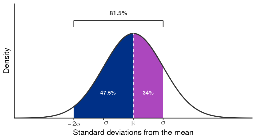
For a normal distribution, which of the following is true?
34% of the distribution lies between \(-2\sigma\) and \(-1\sigma\)
34% of the distribution lies between \(\mu\) and \(2\sigma\)
c) 81.5% of the distribution lies between \(-2\sigma\) and \(1\sigma\)
81.5% of the distribution lies between \(-2\sigma\) and \(2\sigma\)
None of the above
Explanation: The empirical rule states that approximately 68% of the normal distribution lies within 1 standard deviation of the mean, 95% within 2 standard deviations, and 99.7% within 3 standard deviations. \(95/2+68/2=81.5\%\) of the distribution lies between \(-2\sigma\) and \(1\sigma\):