ECON 110: Introductory Economics
Exam 2 Review
Warm-up Quiz 22 10/26
A small town is served by many competing supermarkets, which have the same constant marginal costs.
Using a diagram of the market for groceries, show the consumer surplus, producer surplus, and total surplus.
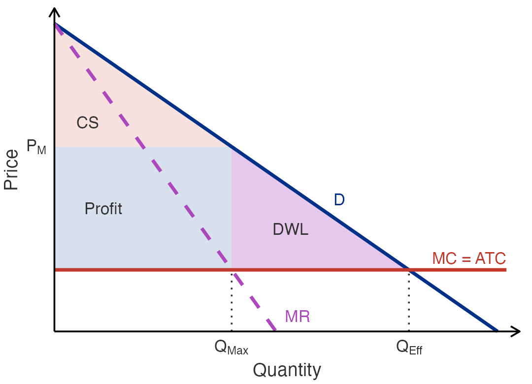
Now suppose that the supermarkets combine into one chain. Using a new diagram, show the new consumer surplus, producer surplus, and total surplus. Relative to the competitive market, what is the transfer from consumers to producers? What is the deadweight loss?
Exam 2 Topics
Exam 2 Review: Chapters 10, 11, and 14
Topics covered:
Chapter 10: Externalities; public solutions; private solutions
Chapter 11: Public goods; common resources; the tragedy of the commons
Chapter 14: The costs of production; explicit versus implicit costs; economic profit; cost curves; short run versus long run; economies of scale
Exam 2 Review: Chapters 15 and 16
Topics covered, continued:
Chapter 15: The competitive firm’s supply decision; shutdown and exit; the market supply curve; long-run equilibrium and zero profit
Chapter 16: Why monopolies arise; the monopolist’s production and pricing decision; the welfare cost of monopoly; antitrust and regulation; price discrimination
Exam 2 Key Concepts
Chapter 10 Key Concepts
- externality
- internalizing the externality
- corrective taxes
- Coase theorem
- transaction costs
Chapter 11 Key Concepts
- excludability
- rivalry in consumption
- private goods
- public goods
- common resources
- club goods
- free rider
- cost–benefit analysis
- Tragedy of the Commons
Chapter 14 Key Concepts
- total revenue
- total cost
- profit
- explicit costs
- implicit costs
- economic profit
- accounting profit
- production function
- marginal product
- diminishing marginal product
- fixed costs
- variable costs
- average total cost
- average fixed cost
- average variable cost
- marginal cost
- efficient scale
- economies of scale
- diseconomies of scale
- constant returns to scale
Chapter 15 Key Concepts
- competitive market
- average revenue
- marginal revenue
- sunk cost
Chapter 16 Key Concepts
- monopoly
- natural monopoly
- price discrimination
Exam 2 Graphs
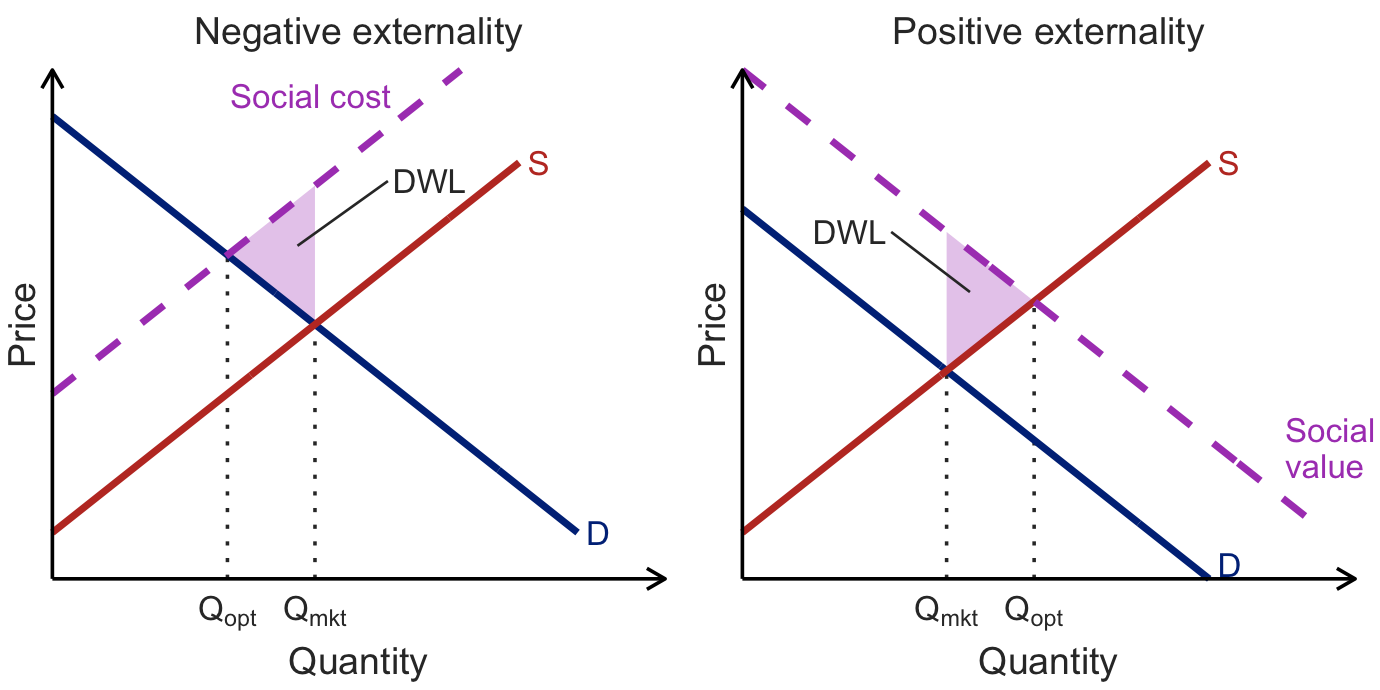
Externalities
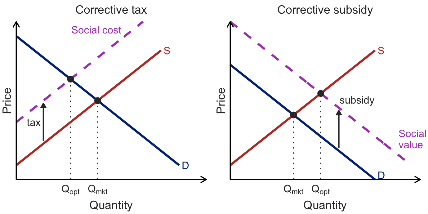
Correcting Externalities
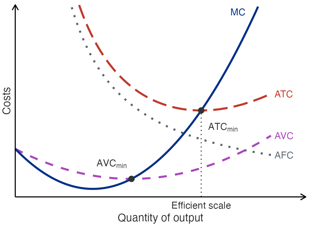
Cost Curves
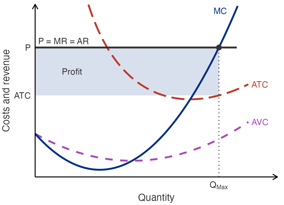
Perfect Competition: Profit
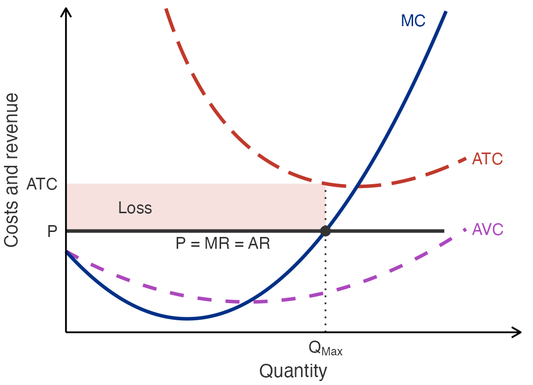
Perfect Competition: Losses
Monopoly: Constant Marginal Cost
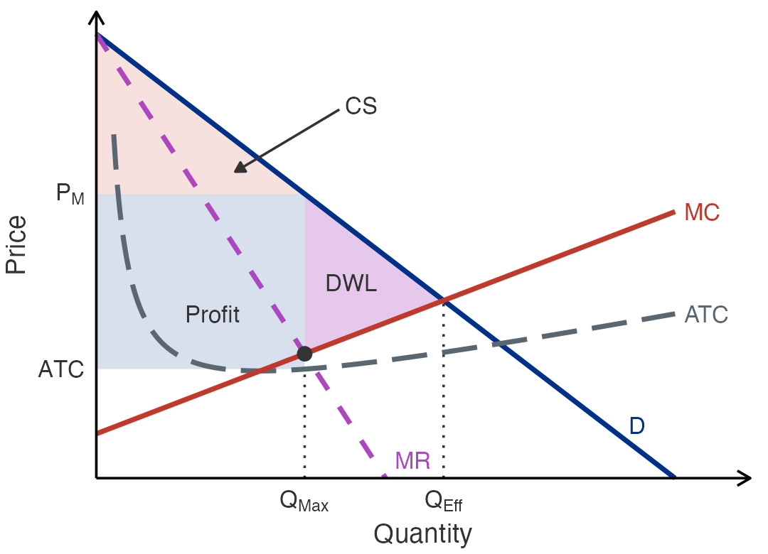
Monopoly: Rising Marginal Cost
Exam 2 Practice Questions
Chapter 10 Practice: Correcting a Negative Externality
In the market for a chemical, demand is \(P = 100 - Q\) and the private cost of production gives supply \(P = 20 + Q\). Each unit produced also causes $20 of pollution damage to people downstream. Find the market quantity, the socially optimal quantity, and the per-unit tax that would move the market to the optimum.
Answer: The market produces 40 units, the optimum is 30 units, and a $20 tax reaches it: \[\begin{aligned} \text{Market: } 100 - Q &= 20 + Q \Rightarrow Q = 40 \\ \text{Optimum: } 100 - Q &= 40 + Q \Rightarrow Q = 30 \end{aligned}\] A tax equal to the external cost makes sellers face the full social cost of each unit.
Chapter 10 Practice: The Coase Theorem
Dev owns a dog that barks at night. Owning the dog is worth $500 to Dev, and the barking costs Dev’s neighbor Mara $800 in lost sleep. If the two can bargain at no cost and Dev has the legal right to keep the dog, what is the efficient outcome, and how could they reach it?
Answer: The efficient outcome is that the dog goes. The barking costs Mara more than the dog is worth to Dev, so Mara can pay Dev any amount between $500 and $800 to give up the dog, and both are better off. The Coase theorem says private bargaining reaches this outcome no matter who holds the legal right.
Chapter 11 Practice: Paying for Streetlights
A town of 1,000 residents is deciding whether to install streetlights that cost $40,000. Each resident values the streetlights at $50. Should the town install them? Why would a private firm be unlikely to provide them?
Answer: Yes. The total benefit is \(1{,}000 \times \$50 = \$50{,}000\), which exceeds the $40,000 cost. A private firm cannot exclude anyone from the light, so each resident has an incentive to free ride rather than pay, and the firm could not collect enough revenue to cover its cost.
Chapter 11 Practice: Classifying Goods
Classify each good as a private good, a public good, a common resource, or a club good:
- Fish in the open ocean
- A streaming video subscription
- National defense
- A slice of pizza
- An uncongested toll road
- Clean air
Answer: Private good: d. Public good: c. Common resources: a and f. Club goods: b and e.
Chapter 14 Practice: Reading a Cost Table
The table shows a food truck’s total cost of producing meals each hour. Find the fixed cost, the marginal cost of the fourth meal, and the average total cost and average variable cost of producing 4 meals.
| Meals | 0 | 1 | 2 | 3 | 4 | 5 |
|---|---|---|---|---|---|---|
| Total cost (USD) | 100 | 150 | 190 | 240 | 300 | 380 |
Answer: Fixed cost is $100, the total cost of producing nothing. The marginal cost of the fourth meal is \(300 - 240 = \$60\). Average total cost is \(300/4 = \$75\), and average variable cost is \((300 - 100)/4 = \$50\).
Chapter 14 Practice: Accounting Versus Economic Profit
Rosa leaves a job paying $60,000 a year to open a bakery, funding it with $100,000 from savings that had been earning 5 percent interest. In the first year the bakery earns $250,000 in revenue and pays $180,000 for ingredients, rent, and wages. Compute the bakery’s accounting profit and economic profit.
Answer: Accounting profit is \(\$250{,}000 - \$180{,}000 = \$70{,}000\). The implicit costs are the forgone salary and the forgone interest, \(\$60{,}000 + \$5{,}000 = \$65{,}000\), so economic profit is \(\$70{,}000 - \$65{,}000 = \$5{,}000\).
Chapter 15 Practice: Choosing Output
A competitive firm sells its output at the market price of $10. Its total costs are shown below. How many units should it produce, and what is its profit?
| Quantity | 0 | 1 | 2 | 3 | 4 | 5 | 6 |
|---|---|---|---|---|---|---|---|
| Total cost (USD) | 8 | 12 | 15 | 20 | 27 | 36 | 47 |
Answer: 5 units, for a profit of $14. Marginal cost is 4, 3, 5, 7, 9, and 11 for units 1 through 6. The firm produces every unit whose marginal cost is at most the $10 price, so it stops at 5 units: profit is \(5 \times \$10 - \$36 = \$14\).
Chapter 15 Practice: Moving to Long-Run Equilibrium
In a competitive industry, every firm has the same cost curves, with minimum average total cost of $8 at 100 units of output. The market price is currently $12. What happens in the long run to the number of firms, the market price, and each firm’s economic profit?
Answer: Firms are earning economic profit at $12, so new firms enter. Entry shifts the market supply curve to the right and pushes the price down until it reaches $8, the minimum of average total cost. At that point each firm earns zero economic profit and entry stops.
Chapter 16 Practice: The Monopolist’s Choice
A monopolist faces the demand schedule below and has a constant marginal cost of $7 with no fixed cost. What quantity does it produce, what price does it charge, and what is its profit?
| Quantity | 1 | 2 | 3 | 4 | 5 |
|---|---|---|---|---|---|
| Price (USD) | 18 | 16 | 14 | 12 | 10 |
Answer: 3 units at $14, for a profit of $21. Total revenue is 18, 32, 42, 48, and 50, so marginal revenue is 18, 14, 10, 6, and 2. Marginal revenue exceeds the $7 marginal cost through the third unit but not the fourth, and profit is \(3 \times (\$14 - \$7) = \$21\).
Chapter 16 Practice: Price Discrimination at the Movies
A theater with 200 empty seats and no marginal cost per ticket can sell to 100 students, each willing to pay $8, and 100 adults, each willing to pay $14. What price maximizes revenue if the theater must charge everyone the same price? How much revenue can it earn if it charges each group a different price?
Answer: With a single price, $8 earns \(200 \times \$8 = \$1{,}600\), which beats \(100 \times \$14 = \$1{,}400\). Charging students $8 and adults $14 earns \(\$800 + \$1{,}400 = \$2{,}200\). Price discrimination raises profit by $600, and every buyer still attends, so it creates no deadweight loss here.