ECON 672: Economics of Development
Week 2: The state of development
Logistics
(Roadmap at the end of slide deck)
Interest surveys have been submitted; I have now connected pairs who reported similar research interests.
Initial project proposals are due on Friday; please plan a discussion with your potential partner, if applicable, and let me know if you are planning to work together.
Print copy of the textbook for loan coming soon!
Lecture Material
What Our Metrics Tell Us
We have previously identified ways to quantify and measure development, but what do these metrics tell us?
We also acknowledged that national output, GNI and GDP, are not complete measures of wellbeing and growth in a country. However, it is primarily these measures (GDPpc) we will first use to discuss the state of development.
However, we should be careful to distinguish income growth from income level; fast growth does not necessarily mean levels of income are equal between two places.
Two Groups and the Distribution of World Income
Two main groups:
“Convergence club” of East Asia, the Pacific, and South Asia, especially China and India, catching up to HICs
Other LMICs, sub-Saharan Africa, Middle East, North Africa, and Latin America, failing to catch up
How is income distributed?
HICs with 17% of population but 65% of world income
LMICs with 83% of the population but 35% of world income
1-5-1 billion populations in LICs, MICs, and HICs (Collier, 2007) with 1-34-65 income split
The Population Tax on Growth
How does population growth affect economic growth?
Remember that \(GDPpc=GDP/N\), such that a faster population growth rate slows down growth in GDPpc holding GDP constant: \[\ln\left(\frac{GDP}{N}\right)=\ln(GDP)-\ln(N)\]
Faster population growth in Africa and slower population growth in Europe and Central Asia means GDPpc is growing similarly (~2%) even if GDP overall is growing much faster in the former region.
We call this the population tax on growth.
GDP Growth and the Population Tax by Region
| Region | GDP | Pop. | GDPpc | Pop. tax |
|---|---|---|---|---|
| South Asia | 6.6 | 1.5 | 5.0 | 23.0 |
| Sub-Saharan Africa | 4.8 | 2.7 | 2.0 | 56.8 |
| East Asia and the Pacific | 4.5 | 0.7 | 3.7 | 16.4 |
| Middle East and North Africa | 3.9 | 2.0 | 1.9 | 51.2 |
| World | 2.9 | 1.2 | 1.7 | 42.4 |
| Latin America and the Caribbean | 2.7 | 1.2 | 1.4 | 45.9 |
| Europe and Central Asia | 1.9 | 0.3 | 1.6 | 17.6 |
Growth Volatility and Initial Income
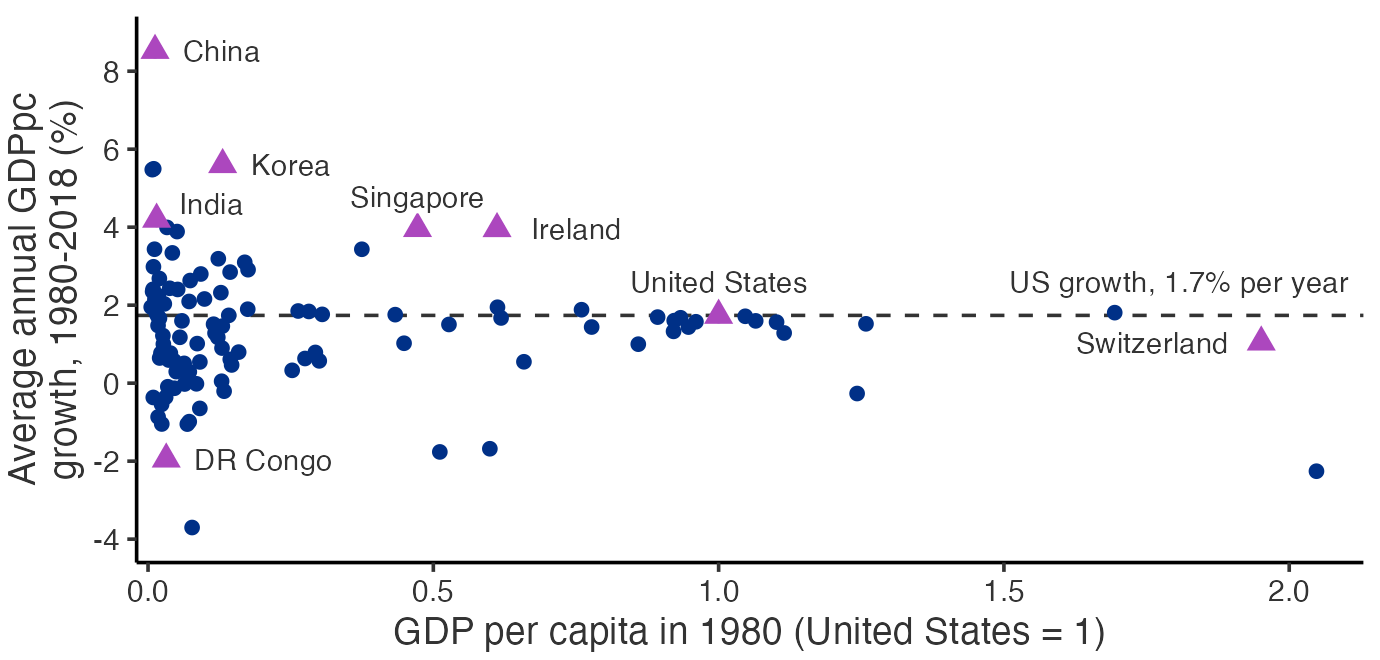
Income growth volatility appears correlated with initial GDPpc:
Metrics We Consider for Development
What metrics do we consider for development?
GDP and GDPpc level and growth
Population growth and fertility
Volatility of growth and income
Poverty (lines), nutrition, hunger, food prices
Geography of growth, poverty, and hunger
Rural Poverty and the Agricultural Sector
…any attempt at reducing world poverty must first and foremost focus on the rural sector, one reason why the performance of agriculture is so important for poverty reduction in the developing world…rural populations must be prepared to migrate successfully out of poverty instead of transposing poverty from the rural to the urban population. This requires investing in their human capital, while rural education has typically lagged far behind urban achievements. The rapid rise of urban slums testifies to this lack of preparedness of rural people when they reach urban labor markets.
— de Janvry & Sadoulet, p. 62
Measuring Inequality
Average income levels hide inequality! How do we measure this?
Gini coefficient: 0-100 for perfect income or wealth equality to perfect inequality
Kuznets inverted-U curve: a negative parabolic relationship we observe between income per capita and income inequality
Growth rates of the Gini coefficient: capture how inequality is changing over time along with income growth
How World Inequality Has Changed
How has world inequality changed over time?
Growth produces inequality (e.g. China, Vietnam) but social programs can redistribute growth and reduce inequality (e.g. Brazil). Both markets and governments have roles to play.
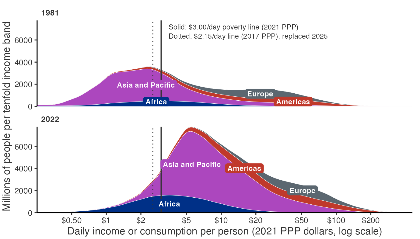
Incomes grew and inequality fell in all regions between 2000 and 2008, showing temporary convergence is possible.
Income growth was generally concentrated in populous countries (e.g. China, India), leading to a fall in population-weighted inequality. This growth lifted huge numbers out of poverty, leading to the rise of a new global middle class.
The World Distribution of Income
Basic Needs: Health and Education
We also consider basic needs, health and education. Here we observe more progress than with GDPpc but still not perfect convergence.
Bounded vs. unbounded outcomes may drive some differences
Life expectancy and education catching up, infant mortality less so
Policy priorities in funding public services matter in addition to income growth
Sustainability and the Emissions Tradeoff
Is growth sustainable?
Food, funding, climate vulnerabilities
Rising energy and water usage (from AI)
Resource scarcity, deforestation, and environmental damage
Negative externalities from growth
Emissions-growth tradeoff:
If growth requires large emissions, should developing countries be allowed to pollute in order to catch up?
Who bears responsibility for cutting their emissions most quickly or sharply?
Multidimensional Quality of Life
Multidimensional measures for quality of life:
Happiness generally correlates with income, World Happiness Report and World Values Survey, but at higher levels of income other factors matter
Institutional and government quality determines corruption levels, public service provision, property protections, and more factors critical for growth
Democratic freedoms expanded and armed conflict and violence declined after the Cold War, all positive for growth, though both trends have reversed since the mid-2010s
Explaining Uneven Convergence
How can we explain this uneven economic convergence we observe?
We will briefly1 consider several models of growth at the macro level, across entire economies.
Generally these models include:
factors of production: land, labor, capital inputs
a production function: turns inputs into output
factor productivity: scaling how technology, institutions, and factor quality in production change over time
Models: Criteria and Components
What makes a good economic model?
Simplification of messy reality but still useful
Unnecessary complexity is eliminated in favor of tractability
Assumptions (sometimes strong) are made and reassessed
Positive and normative analysis can be conducted
Components of a model:
Exogenous variables, policy instruments and environment
Endogenous variables, outcomes of interest
Functional forms for behavior, technology, or institutions
Harrod-Domar and Solow
General models of growth:
Harrod-Domar: post-Great Depression; saving, foreign aid, and constant marginal product of capital drives growth!
Solow: post-HD; decreasing marginal product of capital leads to a steady state conditional convergence; [total] factor productivity (TFP) drives growth!
These models consider:
Capital and labor used in the production process
Investment equal to savings, determined by a savings rate
Constant capital depreciation and population growth
Limits of These Growth Models
Limits of these models:
Endless borrowing to fund endless capital lead to debt crises
Where does TFP growth come from? Backwardness advantage?
Universal convergence does not hold in the data; conditional convergence appears to
Other factors besides population growth, saving, depreciation, and TFP likely affect growth
We do not see labor and financial capital chasing faster growth and higher returns in LDCs (Lucas paradox)
5-minute Break
Acemoglu, Johnson, & Robinson (2001)
Randomly selected presenter: Steph
What is the research question?
How do the authors answer it?
What do they find?
Are you convinced by the design and results?
How does the paper connect to our other readings?
Instrumental Variables (IV) Approach
This paper (and most other papers) wants to estimate the causal impact of some \(X\) on some \(Y\), but faces the problem that variation in \(X\) is not exogenous or (as-good-as) randomly determined.
One method to address this is to find some variable \(Z\) that is correlated with \(X\) and affects \(Y\) only through \(X\). If we first regress \(X\) on \(Z\) and then use the predicted values of \(X\) to estimate the effect on \(Y\), we can isolate the causal effect of \(X\) on \(Y\). This approach is called instrumental variables (IV) estimation2 and \(Z\) is called an instrument.
This approach relies on two key assumptions:
Relevance: \(Z\) is correlated with \(X\) (we can test this)
Exclusion restriction: \(Y\) is not affected by \(Z\) except through \(X\) (we cannot exhaustively test this)
Instrumental Variables in AJR (2001)
The authors ask how much a country’s institutions shape its income today, across a sample of 64 former colonies. Regressing income on institutions directly will not answer this, since richer countries may also be able to afford better institutions.
\(Y\): log GDP per capita in 1995, PPP basis
\(X\): protection against expropriation risk
\(Z\): log mortality rates faced by Europeans in the colonies
Relevance: where disease killed European settlers, colonizers extracted resources rather than settling, and those early institutions persist into the present.
Exclusion restriction: the diseases that killed Europeans, mainly malaria and yellow fever, were far less deadly to local populations who had acquired immunity, so settler mortality is unlikely to be correlated with the health burden a country carries today.
Group Discussion
Bringing together our lecture material and academic article, I have prepared the following suggested discussion questions:
What factors shape development? How might policy be designed to improve growth? Where might it fail?
What measures are used to discuss “development”? Are these measures comprehensive given what we discussed last week? What are their limitations?
We often talk about “good institutions” as a vital ingredient of development; how might we define such “good institutions” and why might these matter so much for development?
Roadmap
Looking Ahead to Week 3
What do we have on the horizon before next Tuesday?
Our Initial Topic Proposals assignment will be due on Friday at 6pm to identify prospective topics for the final project
My office hours for ECON 672 will be held Tuesday before class, 12:15-2:15pm in MCL 108 or virtually by appointment
Our third topic will be Structural transformation and inequality. Our textbook reading will be Chapter 8, pp. 230-244 and Chapter 6. Our required journal article will be Gollin, Lagakos, & Waugh (2014), “The Agricultural Productivity Gap,” QJE.
Our Weekly Reading Response assignment for this paper will be due Tuesday at 2:40pm before class. One student will be randomly selected to present their response to the class in 5-8 minutes.
Footnotes
We will not cover the structural form or solution to these models here. However, I recommend trying to solve these models yourself, starting on p. 220.↩︎
We implement this two-stage process using Ordinary Least Squares (OLS), and thus call this type of IV estimation two-stage least squares or 2SLS.↩︎