ECON 672: Economics of Development
Week 3: Structural transformation and inequality
The Lorenz Curve and the Gini Coefficient
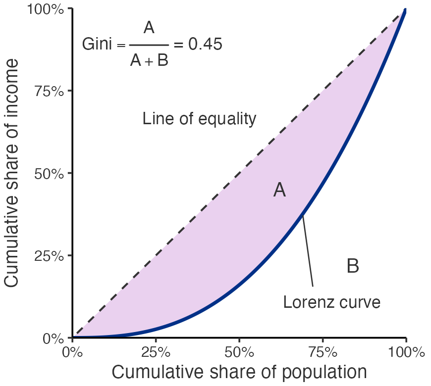
Last time we thought about the Gini coefficient; the Lorenz curve is a graphical representation of this concept.
The Lorenz Curve plots the cumulative share of income (or wealth) against the cumulative share of the population, starting with the poorest individual or household. The further the Lorenz curve is from the line of equality (the 45-degree line), the greater the inequality.
The Gini coefficient can be calculated as the area between the line of equality and the Lorenz curve, divided by the total area under the line of equality.
Lorenz Curve for a Hypothetical Country
The Kuznets Inverted-U Hypothesis
We also thought about the Kuznets curve, an inverted-U-shaped relationship between income inequality and economic development across countries.
We might use Kuznets’s hypothesis to eschew redistributive policies for growth-first policies, since inequality could be seen as a “self-righting” problem. In practice, however, we do not observe a causal relationship between growth and inequality within countries; growth past a certain point does not mechanically lead to lower inequality.
Inequality and Growth in Brazil
In countries like Brazil, inequality rose and fell as GDPpc increased, but the decline has not been due to growth alone, but to social policies introduced by the Cardoso and da Silva governments to reduce inequality.
— de Janvry & Sadoulet, p. 172
Dimensions of Growth
Dimensions of growth:
- Previous models (Harrod-Domar, Solow) discussed GDP(pc) growth, production in the economy as a whole.
- We might also consider (and model) sectoral growth, i.e. growth in agriculture, industry, and services, separately. We general observe that countries transition from agriculture to industry and services as they develop. This is called structural transformation. This is often accompanied by an increase in rural-urban migration.
- However, we should be cautious not to overstate the direction of causality; structural transformation is a consequence of development, not a cause. Simply observing declining agricultural labor shares and rural-urban migration is not always associated with GDP(pc) growth.
Dual-Economy Models
What do these dual-economy models look like?
- Different production functions: capital is an input for industry, land is an input for agriculture; workers are an input for both.
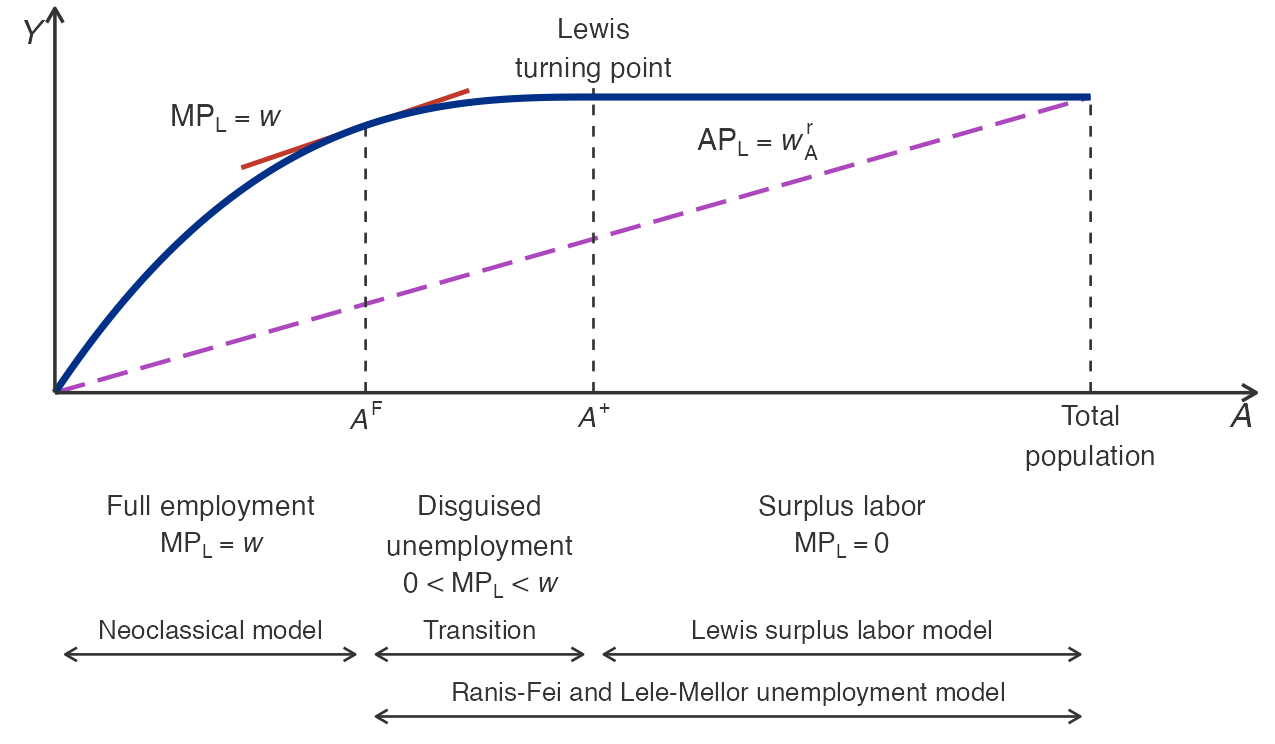
- Lewis: excess labor in agriculture (“disguised unemployment”) can be moved to industry without reducing agricultural output past a certain “turning point”. Higher population growth pushes this point further out, keeping workers in poverty and delaying industralization.
- Empirical estimates of the marginal product of labor in traditional agriculture are often very low, consistent with the idea of “disguised unemployment” and a “dual economy”, but this model is not without its critics.
Agriculture as a Labor Reservoir
…agriculture can serve as a reservoir for surplus labor for a long time, especially if there is population growth, and that for as long as surplus labor exists growth can occur rapidly through investment in industry…The role of agriculture is passive, providing food and labor to industry without the need to invest in agriculture. The model thus justified neglecting agriculture and legitimized a strong “urban bias”.
— de Janvry & Sadoulet, p. 233
Surplus Labor and the Lewis Turning Point
Achieving Long-Term Growth
How is long-term growth achieved in these models?
- Growth in total factor productivity or TFP in agriculture to allow workers to flow from agriculture to industry
- Steady food prices and wages to keep the economy from stagnating
- Movement of workers between sectors, likely rural to urban
- China 1978–1984 example: rapid productivity growth in agriculture, stable food prices, labor moving to industry1
Dual economy models after Lewis:
Jorgenson (1967)
Ranis & Fei (1961) and Lele & Mellor (1981)
Endogenous Growth and Total Factor Productivity
Problem: so what IS total factor productivity, the key to growth?
- Romer (1990) model of endogenous growth: I can choose to invest labor in research as well as final production and this in turn benefits productivity. We now treat this Cobb-Douglas “A” as an endogenous factor of production.
- Ideas are protected using patents, making them excludable but non-rival. That is, you using my idea to make something does not stop me from using it (non-rival), but I can legally prevent you from using my idea for a period of time (excludable). Otherwise, I have no incentive to invest in research!
- These labor-saving ideas will yield increasing returns to scale, meaning we do not predict convergence. Instead, Romer’s model predicts a balanced growth path (BGP) and labor moving from LDCs to MDCs, accelerating divergence.
The Agricultural Productivity Gap
Agricultural productivity gap: average value added per worker is lower in the agricultural sector than in industry, particularly in developing countries. We call this a misallocation of labor2.
What should workers do? Move from agriculture to industry! We broadly call this structural transformation.
GLW (2014) study if this perceived gap is coming from mismeasurement and largely conclude no. Instead, their evidence suggests that the persistence of this gap may come from poor institutional quality, geography, or labor mobility. These are all factors of development we have or will consider more deeply.
Takeaways from the Misallocation Story
Key takeaways of this labor misallocation story:
- People have different levels of skill; some of these skill differences may be person-based, such as education and experience, others place-based, such as local infrastructure and market access, and others sector-based, i.e. specific skills.
- A simple economic model would predict workers move to the sector where they are most productive (highest value added). However, this requires the ability and willingness to migrate, among other things.
- If workers do not move to sectors/areas where they provide the highest value added, aggregate (country-level) productivity and growth suffers. In reality, we do see this productivity gap between sectors persist: higher potential gains are not pulling enough workers out of agriculture, particularly in developing countries (or sorting is on unobservable skill, e.g. Young 2013).
Why the Agricultural Divide Matters
McMillan and Rodrik (2011) argue that reallocations of workers to the most productive sectors—taking the underlying productivity data at face value—would raise aggregate output per worker substantially in many countries.
Our focus on the divide between the agricultural and nonagricultural sectors is important because the vast majority of workers in developing countries are in agriculture…
— Gollin, Lagakos, & Waugh, 2014, pp. 942–943
The Cobb-Douglas Production Function
Cobb-Douglas production function: \[Y_j=A_jL_j^\alpha K_j^\beta\]
\(Y_j\) is output in sector \(j\)
\(A_j\) is total factor productivity (TFP) for output in sector \(j\)
\(L_j\) is the labor input in sector \(j\) and \(K_j\) is the capital input
\(\alpha\) and \(\beta\) are the output elasticities of labor and capital, i.e. the percent increase in output from a one percent increase in workers or machines. \(\alpha<1\) and \(\beta<1\) imply diminishing marginal returns to labor and capital, respectively.
\(\alpha+\beta=1\) implies constant returns to scale (CRS); doubling all inputs (capital \(K\) and labor \(L\)) should double output \(Y\). \(\alpha+\beta<1\) implies decreasing returns to scale; \(\alpha+\beta>1\) implies increasing returns to scale. We generally assume CRS.
5-minute Break
Gollin, Lagakos, & Waugh (2014)
Randomly selected presenter: Emily
What is the research question?
How do the authors answer it?
What do they find?
Are you convinced by the design and results?
How does the paper connect to our other readings?
Group Discussion
Bringing together our lecture material and academic article, I have prepared the following suggested discussion questions:
What do we mean by “structural transformation” in an economy? How does this relate to a story of economic growth? Who might be the winners and losers from such a transformation?
What do we mean by “labor misallocation”? How does this relate to structural transformation and economic growth?
Based on the models we have discussed, what might be the key to sustained economic growth? What are the key constraints to achieving this growth? Should we expect growth to be distributed equally among the population?
Roadmap
Looking Ahead to Week 4
What do we have on the horizon before next Tuesday?
My office hours for ECON 672 will be held Tuesday before class, 12:15-2:15pm in MCL 108 or virtually by appointment
Our fourth topic will be History of thought in development economics. Our textbook reading will be Chapter 3. Our Poor Economics reading will be the Foreword and Chapter 1. Our required journal article will be Rodrik (2010), “Diagnostics before Prescription,” JEP.
Our Weekly Reading Response assignment for this paper will be due Tuesday at 2:40pm before class. One student will be randomly selected to present their response to the class in 5-8 minutes.
Footnotes
Really this was a case of industry moving to labor due to the Hukou labor-registration system during this period limiting migration.↩︎
We would analogously call a mismatch in value added per machine a misallocation of capital. Authors such as Hsieh & Klenow consider this gap between firms, while others such as Caselli & Feyrer study the gap between countries.↩︎
Let \(\pi=Y-wL-rK\) represent real net profits, output less labor and capital costs. Profit-maximizing firms set \(\partial\pi/\partial L=\partial Y/\partial L-w=0\), or \(\partial Y/\partial L=w\). Assuming CRS, \(Y=AL^\alpha K^{1-\alpha}\), \(\partial Y/\partial L=\alpha A(K/L)^{1-\alpha}\). Thus, the labor share \(wL/Y=(\alpha A(K/L)^{1-\alpha}L)/(AL^\alpha K^{1-\alpha})=\alpha\).↩︎