ECON 672: Economics of Development
Week 5: Impact evaluation
Disclaimer
Warning: \(\underbrace{\text{econo}}_{\scriptscriptstyle\text{economics}}\overbrace{\text{metrics}}^{\scriptscriptstyle\text{measurement}}\) ahead
Decorative figure: a scatterplot of observations with an upward-sloping fitted regression line drawn through them.
Banerjee & Duflo on the Spread of RCTs
The number of completed RCTs1 within J-PAL2 went from 327 in 2008 to more than 2,204 in 2024, and other organizations, including the World Bank, the Inter-American Development Bank, and many others, also added trials of their own…Many of those who had initially expressed skepticism about the value of field experiments, and others who were simply busy with other work, seemed taken by the new insights that were coming out of the RCTs and decided to dip their feet in. Other fields of economics, focused on rich countries rather than the developing world where we were doing most of our work, also discovered or rediscovered the joy of experimentation and brought in a whole slew of new talent.
— Banerjee & Duflo, p. x
What Impact Evaluation Is For
Impact evaluation identifies causal effects3 of a program on relevant outcomes
Accountability and ex-post cost-benefit analysis of causal impacts for financers by external evaluators
Results-based management using evidence to tweak or overhaul design for subsequent phase or scale-up (or cancelation)
General lessons for the field as a public good (e.g. work on conditional cash transfers or CCTs)
The Potential Outcomes Setup
Setup:
Causal impact \((\delta)\) of program \(P\in\{0,1\}\) on outcome \(Y\), for units \(i\in\mathsf{n}\subset\mathsf{N}\), our sample4 within the population5
Ideal: \(\delta_i=Y_i(1)-Y_i(0)\)
Constraint: the counterfactual, or what outcomes would have looked like without the program, is unobservable
Reality: take averages6 across units: \[\delta=\underbrace{E[Y_i(1)-Y_i(0)]}_{\text{Average difference in outcomes}}=\underbrace{E[Y_i(1)]-E[Y_i(0)]}_{\text{Difference in average outcomes}}\]
Causal Methods for Impact Evaluation
Causal methods:
Randomized controlled trials (RCTs), the gold standard of impact analysis, assume generalizability and exogeneity and so may still face problems (Deaton, 2010)
Matching methods including propensity score matching (PSM) that construct comparable groups on observables, assuming unobservables are also comparable. This delivers the treatment on treated (ToT) estimate, the average difference in outcomes between treated participants and matched non-treated, non-participants7.
Causal Methods: Differences and Panels
Causal methods pt. 2:
Difference-in-difference (DiD) compares changes in outcomes before and after a program for treated and untreated groups, assuming parallel trends: \[ATE=\Delta E[Y_T]-\Delta E[Y_C]=\left(\bar{Y}_{T1}-\bar{Y}_{T0}\right)-\left(\bar{Y}_{C1}-\bar{Y}_{C0}\right)\]
Panel analysis or staggered dif-in-dif compares program rollout with heterogeneous timing, assuming no changes in context or behavior between units over time outside of program8
Event study compares outcomes many periods before and after a policy change for treated and untreated units
Causal Methods: Discontinuities and Instruments
Causal methods pt. 3:
Regression discontinuity (RD) compares units just above and below a threshold (e.g. Dell, 2010), assuming no sorting and smoothness over threshold. Under sharp RD the threshold is fully binding, so assignment perfectly predicts take-up; under fuzzy RD it is only mostly binding, so assignment serves as an instrument for take-up
Instrumental variables (IV) approach rescales variation in an endogenous independent variable by an exogenous instrument (e.g. Acemoglu, Johnson, & Robinson, 2001)
Natural experiments are rare but sometimes present themselves, where nature (or policy) has already randomized assignment (e.g. Chattopadhyay & Duflo, 2004)
Experimental Design and the Average Treatment Effect
Experimental design:
Ethics9 of choosing control group, non-deception, non-compliance, and withdrawal of consent
Average treatment effect (ATE) can be estimated as \(ATE=\bar{Y}_T-\bar{Y}_C\). Our ATE is statistically significant if our two means are significantly different10
Conditional average treatment effect (CATE) is the ATE for specific values of observables \(X\), \(CATE=\left(\bar{Y}_T-\bar{Y}_C\right)\mid X\)
Ordinary Least Squares
Regression is a central tool in empirical economics to estimate relationships between variables, and to test hypotheses about them:
We are interested in the true relationship between an outcome and one or more predictors in a population, but we observe only sample(s), so we must estimate the effect. We call using sample estimates to learn about the population inference; whether those estimates recover the true effect we care about, rather than a biased one, we call identification.
Ordinary Least Squares (OLS) is a common method of estimating this (linear) relationship by minimizing the sum of squared residuals, deviations between observed and predicted outcome values, across sample observations.
Bias and the Standard Error
Key properties of OLS estimation:
Our estimator is unbiased if it is correct (equal to the population value) on average across samples, and consistent if it converges to the truth as the sample size grows.
Our estimator’s standard error estimates how much our estimate would vary from sample to sample. We use this for constructing confidence intervals and hypothesis testing, so an incorrect standard error leads to improper inference.
Note that using OLS does not necessarily deliver a causal estimate of the relationship between predictor(s) and outcome; this requires additional assumptions.
Randomized Controlled Trials
RCTs are a workhorse tool of development economics: by randomly assigning units to treatment or control, we may estimate a causal treatment effect.
But the field is messy, and even a carefully designed experiment can face problems that threaten its validity.
Today we cover common threats to RCT designs and how to address each, whether we are designing an experiment or evaluating one. We organize these broadly around two questions:
Is our estimate right? Non-compliance, spillovers, and attrition can bias our estimate of the effect (a problem of identification); external validity asks whether it generalizes.
Is our uncertainty right? Clustering deflates our standard errors, multiple hypothesis testing inflates false positives, and low power hides true effects, all problems of inference.
Seeds and Crop Yields
Suppose a development agency wants to know whether a new experimental seed technology raises farmers’ crop yields.
We randomly assign farmers to treatment (the new seed) or control (their usual seed), and measure each farmer’s yield during harvest:
\[ \begin{aligned} Y_i &= \beta_0 + \delta P_i + \beta_1 X_{1i} + \cdots + \varepsilon_i \quad\text{(population)}\\ Y_i &= b_0 + d P_i + b_1 X_{1i} + \cdots + e_i \quad\text{(sample)} \end{aligned} \]
Here \(Y_i\) is farmer \(i\)’s yield, \(P_i\) indicates the program, \(\delta\) is the true causal effect, and \(d\) estimates the seed’s causal effect in the sample (unbiased under proper randomization)11.
Hypothesis Testing and the p-value
Estimating an effect is not the same as establishing that there is one, so we frame the question as a hypothesis test:
The null hypothesis \(H_0\) says there is no effect, \(\delta=0\), and the alternative \(H_1\) says there is one, \(\delta\neq 0\).
Our test statistic rescales the estimate by its standard error, \(t=\frac{d}{s_d}\), asking how many standard errors our estimate sits away from the null.
The p-value is the probability of seeing an estimate at least this extreme if the null were true. A small p-value means our data would be surprising in a world with no effect.
We reject the null when the p-value falls below a chosen significance level \(\alpha\), conventionally 5%. Failing to reject is not evidence of no effect; we may simply lack the power to detect one.
Why Randomization Helps
Random assignment aims to make the treatment and control groups comparable from the start: because treatment is decided purely by chance, it is unrelated to any farmer-specific factors, observed or unobserved.
This means \(P_i\) is uncorrelated with the error term, and \(d\) is an unbiased, consistent estimate of the average treatment effect.
Even valid randomization is not airtight (Deaton, 2010). Hawthorne and John Henry effects, where farmers behave differently because they are observed or untreated, and experimenter demand effects, where farmers offer the outcomes they perceive we are looking for, can both bias \(d\); blinding and unobtrusive measurement help.
The threats that follow are the ways this clean result breaks down in the field. They either bias \(d\), a problem of identification, or leave \(d\) unbiased while undermining the inference we draw from it.
Checking Balance
Balance checks. Before trusting our estimate \(d\), we confirm randomization actually produced comparable groups by comparing pre-treatment characteristics across arms: baseline plot size, soil quality, and prior yield.
Sharp differences suggest the random assignment failed or was compromised; we can then control for these covariates or investigate further.
With many covariates, though, we would expect some to look different purely by chance, roughly 5% of them when we test at the 5% level, so we typically judge balance with a joint test rather than variable by variable.
Balance on observables is reassuring but not decisive: randomization is what secures balance on unobservables, in expectation.
Non-compliance
Non-compliance. In the field, not everyone assigned to treatment (\(P_i\)) actually takes it up (\(W_i\)). Suppose only the most experienced farmers plant the new seed when assigned to treatment.
Comparing those who actually used the seed against everyone else no longer compares randomly assigned groups, so \(d\) is biased by who chose to comply.
We call those who always take up the program regardless of treatment assignment always-takers (\(W_i=1\) always), while those who never take up the program are never-takers (\(W_i=0\) always). Compliers are those who behave as assigned (\(W_i=P_i\)) while those who behave opposite from assignment are defiers (\(W_i=1-P_i\) for \(W_i,P_i\in\{0,1\}\)).
Non-compliance: ITT and LATE
Two methods keep randomization intact under non-compliance:
- Intention-to-treat (ITT): compare groups by their original assignment, ignoring take-up. This measures the effect of being offered the seed, often the policy-relevant question.
- Local average treatment effect (LATE): use assignment as an instrument (a nudge that shifts take-up but affects yields only through it) to recover the effect of using the seed, for the (“local”) compliers who adopt only when assigned.
A randomized encouragement design uses the same idea when treatment cannot be randomized (e.g. program is already available but has low take-up), as long as the nudge never pushes anyone the opposite way12 (we call this condition monotonicity or “no defiers”).
Spillovers and SUTVA
Spillovers (interference). Our comparison assumes one farmer’s treatment does not affect another’s outcome: the Stable Unit Treatment Value Assumption (SUTVA), specifically the no-interference part13.
But if treated farmers share their seed, or what they learn, with neighbors (peer effects), the control group becomes partly treated.
This spillover shrinks the gap between groups and biases our estimate toward zero14.
Spillovers: Design Fixes
We can limit spillovers at the design stage, through how we set up the experiment:
Randomize whole villages instead of individual farmers, so spillovers stay within units
Vary the share treated across villages to measure spillovers directly and include this in the analysis (Baird et al., 2018)
Introduce buffer zones between areas to limit spillover contamination
Attrition
Attrition bias. Some farmers may also drop out of the sample before we measure their yields: they migrate, refuse follow-up surveys, or cannot be found.
If attrition is differential, tied to both treatment and outcome, the remaining sample is no longer randomly assigned.
If discouraged treated farmers leave, the treated who remain look unusually successful, and \(d\) overstates the true effect.
Attrition: Corrections
ITT/LATE does not fix attrition; it still needs an outcome for everyone, which is exactly what is missing. Instead we can:
Recover it by intensively tracking and re-surveying a (random sub)sample of those lost.
Bound it with Lee (2009) bounds: if drop-out runs one way, trim the better-retained group to the other’s response rate, giving a worst-to-best-case range.
Reweight survivors to stand in for similar dropouts based on their predicted likelihood of attrition (inverse-probability weighting).
External Validity
Site-selection bias. An RCT cleanly estimates the effect only for the units that took part; whether it generalizes beyond them is a separate question of external validity.
Suppose skeptical, poor-soil villages decline to enroll. Our estimate may still be internally valid, measuring in our design what we think we are measuring for the villages that participated, the identification concern from before. It need not carry over to villages that opted out, or to other regions, times, or implementers.
External Validity: Scale and Remedy
Scale is a second reason our results may not travel (Deaton, 2010). Our treatments usually study one side of a market at a time, so what we recover is a partial equilibrium effect; when the whole economy adjusts, the general equilibrium impact may look quite different.
If every farmer in the region plants the new seed, the harvest glut may push prices down far enough to undo the income gain we measured on a handful of villages.
No estimator fixes either problem; the remedy is at the sampling stage: we choose study sites that resemble our population of interest, and explicitly acknowledge any remaining threats to external validity.
de Janvry & Sadoulet on Validity and Policy
A great deal of attention is given in impact evaluation to internal validity. This consists of showing that the control group has been properly chosen against the treatment group within the selected population of eligible control individuals, households, institutions, or communities. But usefulness for policy purposes requires that results also achieve some reasonable level of external validity with respect to the broader population of eligible individuals, households, institutions, or communities. Establishing the external validity of an impact can be obtained by replicating the experiment over different selections of eligibles, by estimating behavioral parameters (e.g. elasticities), by exploiting heterogeneity in impact, or by planning experimentation across a variety of contexts.
— de Janvry & Sadoulet, pp. 129-130
Banerjee & Duflo on Experiments vs. Non-Experiments
…the concerns about experiments are not new. However, many of these concerns are based on comparing experimental methods, implicitly or explicitly, with other methods for trying to learn about the same thing…Note that, although some of these issues are specific to experiments (we point these out along the way), most of these concerns (external validity, the difference between partial equilibrium and market equilibrium effects, nonidentification of distribution of effect) are common to all microevaluations, both with experimental and nonexperimental methods. They are more frequently brought to the forefront when discussing experiments, which is likely because most of the other usual concerns are taken care of by the randomization.
— Banerjee & Duflo, 2009, p. 159
Clustered Standard Errors
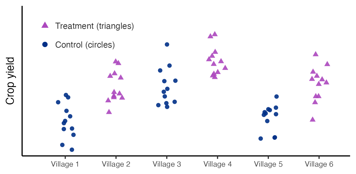
Clustering. Having randomized by village, our estimate may be unbiased but its standard error could now be wrong.
Farmers in a village may share weather, prices, and leadership, so their errors are correlated, while those in different villages may not.
OLS assumes independent errors, so this within-village correlation makes the conventional standard error too small, and we overstate our certainty.
Clustered Standard Errors: Two Caveats
The fix is cluster-robust standard errors, which allow correlation within villages but assume independence across them. Two caveats:
- Independence across clusters must hold: a shared region-wide shock (e.g. war) would force us to cluster at the region level rather than the village level, which may make inference challenging with a small number of regions.
- We need enough clusters: cluster-robust standard errors rely on having many villages (the more the better), with 30 to 50 as a common floor. With fewer, the wild cluster bootstrap15 is the standard fix. We also watch out for thin, unequal, or few treated clusters, which can make inference unreliable.
Within-Village Clustering
Testing Many Outcomes
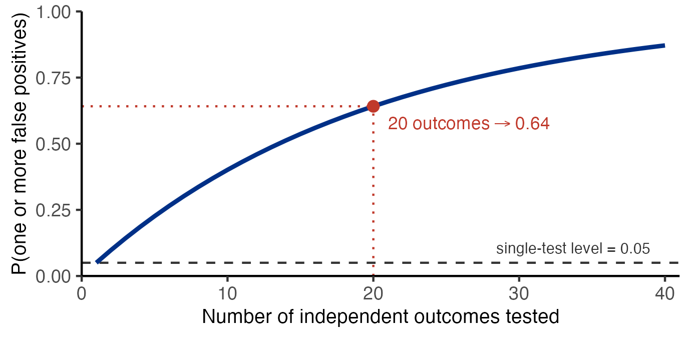
Multiple hypothesis testing. Field experiments typically record many outcomes: yield, plant height, disease resistance, farmer income, and we may want to estimate treatment effects for all of them. Remember that for each hypothesis test, we have an \(\alpha\) chance of a false positive (a significant result when the null is true) when testing at the \(\alpha\) level.
If we test enough at the 5% level, this becomes a serious problem: with 20 independent true nulls, the chance of at least one false positive is \(1-\Pr[\text{No false positives}] = 1 - (1 - 0.05)^{20} \approx 0.64\).
Reporting only the tests that “worked” invalidates our inference.
Testing Many Outcomes: False Positives Multiply
Testing Many Outcomes: Safeguards
With many outcomes, we can protect our inference in three ways:
- Pre-register a pre-analysis plan naming the main outcomes in advance, ruling out p-hacking (searching the data for whatever turns out significant and not reporting nulls).
- Adjust the threshold by applying a correction16 for multiple hypothesis testing that raises the bar for significance as we test more outcomes, keeping the overall false-positive rate in check.
- Aggregate related outcomes into a single summary index, typically an average of the standardized outcomes, so one test replaces many, e.g. “harvest success”.
Statistical Power
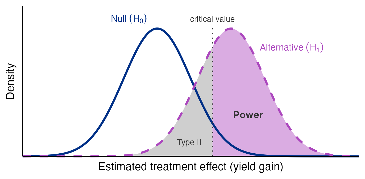
Power is the chance of detecting a real effect when there is one (i.e. the null is false). The minimum detectable effect (MDE) is the smallest true effect a study can reliably detect; researchers often target a specific MDE (e.g. a 10% yield increase) at the design stage, yet can still end up underpowered due to unexpected variation, attrition, or low take-up.
Underpowered studies are doubly dangerous. They usually miss real effects, and because their standard errors are large, only an unusually big estimate can clear the significance bar. So the significant findings that survive overstate the true effect.17
Power also falls as we cluster: correlated farmers add less than one independent observation each, so the number of villages is the more relevant unit of observation. Always run a power calculation before collecting data (many grants will also ask for this and the MDE).
Statistical Power: Power vs. Type II Error
Summary: Designing and Evaluating Field Experiments
To review, we ask two broad questions when we design or evaluate a field experiment:
- Is the estimate right? (identification) Watch for non-compliance (report ITT and LATE), spillovers (randomize at the right level), and attrition (track, bound, or reweight); and consider external validity, whether the effect generalizes.
- Is the uncertainty right? (inference) Cluster at the level of randomization, ensure sufficient clusters, adjust for multiple hypothesis testing, and sufficiently power the study (i.e. recruit a large enough sample) ahead of time.
Famous RCT Designs in Development
Famous RCT designs (many we will read):
Deworming programs for schoolchildren
(Conditional) cash transfers on household incomes
Microcredit and microfinance on entrepreneurs
HIV testing information on sexual health behavior
Improving management practices in firms
de Janvry & Sadoulet on the Black Box
An important limitation of simple impact analyses is their “black box” nature: they provide a measure of the impact of a very specific program in the way it was implemented, but cannot tell us, for example, why people responded the way they did, nor how they would have responded had the level of subsidy been different.
— de Janvry & Sadoulet, p. 113
Deaton on Learning What Works
…my main concern is with how we should go about finding out whether and how assistance works and with methods for gathering evidence and learning from it in a scientific way that has some hope of leading to the progressive accumulation of useful knowledge about development.
— Deaton, 2010, p. 425
Banerjee & Duflo on Waiting for the Spark
…we are largely incapable of predicting where growth will happen, and we don’t understand very well why things suddenly fire up…Given that economic growth requires manpower and brainpower, it seems plausible, however, that whenever that spark occurs, it is more likely to catch fire if women and men are properly educated, well fed, and healthy and if citizens feel secure and confident enough to invest in their children and to let them leave home to get the new jobs in the city. It is also probably true that until that happens, something needs to be done to make that wait for the spark more bearable.
— Banerjee & Duflo, p. 314
5-minute Break
Deaton (2010)
Randomly selected presenter: Oliver
What is the research question?
How do the authors answer it?
What do they find?
Are you convinced by the design and results?
How does the paper connect to our other readings?
Group Discussion
Bringing together our lecture material and academic article, I have prepared the following suggested discussion questions:
We have seen a few of these causal estimation methods in our required and recommended readings; how were they used, what did they assume, and how did they find causality?
How should we reconcile Deaton’s concerns with RCTs against Banerjee, Duflo, and others’ success with them in development economics?
We have previously discussed Rodrik’s caution to tailor interventions to a place in the design and implementation stages of an experiment. Using what we have seen this week, what steps should we also take after an experiment has been done to ensure prudent and valid impact evaluation?
Roadmap
Looking Ahead to Week 6
What do we have on the horizon before next Tuesday?
Our Preliminary Literature List assignment will be due on Friday at 6pm
My office hours for ECON 672 will be held Tuesday before class, 12:15-2:15pm in MCL 108 or virtually by appointment
Our sixth topic will be Poverty, vulnerability, and poverty traps. Our textbook reading will be Chapter 5. Our Poor Economics reading will be Chapter 2. Our required journal article will be Kraay & McKenzie (2014), “Do Poverty Traps Exist? Assessing the Evidence,” JEP.
Our Weekly Reading Response assignment for this paper will be due Tuesday at 2:40pm before class. One student will be randomly selected to present their response to the class in 5-8 minutes.
Appendix: ITT Specification
Let \(P_i\) denote random assignment (1 if offered the new seed) and \(W_i\) actual take-up (1 if the farmer plants it). Under full compliance \(P_i = W_i\), so the \(P_i\) of the main model captures both; under non-compliance they diverge.
Intention-to-treat regresses yield on assignment: \[Y_i = \alpha_0 + \tau_{ITT}\, P_i + u_i\]
Because \(P_i\) is randomized, OLS recovers \(\tau_{ITT}\), the effect of being offered the seed.
Appendix: LATE Specification
LATE instruments take-up \(W_i\) with random assignment \(P_i\) (2SLS): \[\begin{aligned} \text{first stage:}\quad & W_i = \pi_0 + \pi_1 P_i + \nu_i \\[4pt] \text{second stage:}\quad & Y_i = \gamma_0 + \tau_{LATE}\, \hat{W}_i + \xi_i \end{aligned}\]
The second stage regresses yield on the fitted \(\hat{W}_i\), so \(\tau_{LATE}\) uses only assignment-driven take-up. When just-identified18 it equals the Wald ratio \(\tau_{LATE} = \frac{\tau_{ITT}}{\pi_1}\), recovering the effect of using the seed for compliers19.
Appendix: ITT vs. LATE
We may consider whether to report the ITT or LATE estimate; in practice these are often presented together.
ITT measures the direct impact of treatment assignment (e.g. being offered seed) on the outcome, while the LATE rescales this effect by the strength of the first stage20. These both utilize the same identifying variation, but are relevant for different research questions.
We may prefer ITT estimates when considering the effect of a policy as implemented (for always-takers, compliers, never-takers, and defiers), while LATE estimates are more relevant for understanding the effect of actually utilizing the treatment (for compliers21).
Footnotes
Randomized Controlled Trials↩︎
Abdul Latif Jameel Poverty Action Lab↩︎
We distinguish causal effects from correlational findings; whether or not a program is associated with changes in outcomes is much less informative than showing the program caused a difference in outcomes.↩︎
Our sample, indexed from \(i=1,\dots,n\), is ideally representative.↩︎
Our true population, indexed from \(i=1,\dots,N\), may include past, present, future, or hypothetical units and is generally unobservable.↩︎
Because the expectation operator \(E[\dots]\) is linear, the average of differences is equal to the difference of averages.↩︎
We may employ such a design when it is not feasible or ethical to generate a typical control group of untreated units with which to compare treated units.↩︎
Imagine we compare outcomes of a subsidy program delivered either 6 months or 1 year ago; if we believe the transfer sets treated households on a continuous path of income growth, it would not be appropriate to compare early- and late-treated households with a staggered dif-in-dif, as earlier-treated households would have had longer to accumulate additional wealth.↩︎
A key step for any experiment with human subjects is approval by the Institutional Review Board (IRB), which ensures proper consent from, treatment of, and disclosure to subjects before, during, and after the project.↩︎
We typically test mean differences using a t-test at the 5% level or nonparametric Chi-squared test for percentage differences.↩︎
Additionally, \(\varepsilon_i\) and \(e_i\) are the error term and residual, capturing unobserved factors affecting yields in the population and sample, respectively. \(X_{1i}\) is an observable covariate with coefficient \(\beta_1\), and “\(\cdots\)” allows for further covariates. As Deaton (2010) points out, proper randomization should make inclusion of covariates unnecessary to obtain unbiased estimates of \(\delta\), though their inclusion may still improve the precision of \(d\) and thus aid inference.↩︎
Defiers in this case would be farmers who adopt the new seed when assigned to control or vice versa.↩︎
SUTVA also requires no hidden variations of treatment: every treated farmer receives the same, well-defined version of the seed. If instead some experimental seeds were rotten and thus ineffective, this assumption would be violated.↩︎
The direction of bias depends on the spillover’s sign: positive spillovers onto the control group, as here, pull the estimate toward zero, while negative spillovers, such as treated farmers out-competing their neighbors for buyers, can make controls worse off and push the estimate away from zero.↩︎
Bootstrapping generally is a technique of treating the sample as the population and resampling many times with replacement, mimicking the true unobserved sampling process. The wild cluster variant does something slightly different: rather than resampling villages, it re-draws the data by randomly flipping the sign of each village’s residuals.↩︎
One such correction for multiple hypothesis testing is the Bonferroni, a quite conservative adjustment to p-values that often leads to weakly significant results becoming insignificant.↩︎
This selection-driven inflation of statistically significant estimates is known as the winner’s curse, or Type M (magnitude) error (Gelman & Carlin, 2014).↩︎
A just-identified case is one with the same number of instruments (\(P_i\)) as endogenous variables (\(W_i\)).↩︎
Valid under instrument relevance (\(\pi_1 \neq 0\)), the exclusion restriction, and monotonicity (no defiers).↩︎
The first stage is equal to the raw take-up rate only under one-sided non-compliance, e.g. when no farmers in the control group get the new seed.↩︎
Remember that the validity of the LATE estimate relies on the no-defiers assumption, e.g. no farmers who take up the treatment only when assigned to the control group and vice-versa.↩︎