ECON 672: Economics of Development

Week 7: Population, fertility, and the household

Gender Roles in the Household

Gender roles affect intra-household bargaining and decision-making:

• cash crop (male priority) vs. food crop (female priority) land planting allocation

• family plot vs. woman’s own plot fertilizer allocation

• investment (male priority) vs. children’s health, nutrition, and education (female priority) for cash transfers (CTs)

• food allocation among household members, especially during drought or shortages

A Model of Household Decision-Making

For man \(M\) and woman \(F\) in a household, we can specify utility functions \(U_M(q,a)\) and \(U_F(q,a)\) over household consumption amount \(q\) and household actions (e.g. labor supply) \(a\). \(Y_M(a)\) is the income earned by the man’s activities, \(Y_F(a)\) is the income earned by the woman’s activities, and \(T_{M/F}\) are any transfers received by the man or woman.

The household thus maximizes utility: \[\underset{q,a}{\max}\hspace{3pt}U_M(q,a)+\mu U_F(q,a)\] subject to the budget constraint: \[pq=Y_M(a)+Y_F(a)+T_M+T_F\] We notice the \(\mu\) term on the woman’s utility; this governs intra-household allocation of consumption.

Household Bargaining Power

This \(\mu\) term reflects the bargaining power in the household between men and women. We could imagine:

• a unitary model, where \(U_M(q,a)=U_F(q,a)=U(q,a)\), i.e. one member makes decisions for the entire household, there is cooperation, or members have the same utility function (efficient, Pareto optimal)

• a bargaining model where \(\mu\) is set exogenously before the relationship based on the woman’s outside options, including education, labor market opportunities, directly controlled assets, or other independent income (also efficient, Pareto optimal), where \(\mu\) reflects household equity

• a bargaining model where \(\mu\) is set endogenously based on \(q\) and \(a\) (non-separable, not Pareto-efficient); \(\partial\mu/\partial Y_F(a)>0\), \(\partial\mu/\partial T_F>0\) (richer women have more power)

Testing for Income Pooling

We may want to conduct studies to understand what type of utility functions households seem to have that govern their bargaining behavior to understand both existing gender norms and the impacts of future programs, e.g. cash transfers or work programs.

One way we could test these utility models is by looking for income pooling: a transfer given to either the man or woman in either of the first two cases above would be allocated to consumption according to the separable utility function regardless of the recipient: i.e., whether the man or woman received the transfer should not affect how it is used unless \(\mu\) is endogenous.

Evidence Against Income Pooling

Studies including Duflo (2003) have tested this and generally rejected the pooling hypothesis: household bargaining power of women appears to be endogenously determined by activities within the household.

The consequence of these findings is inefficiency in household allocation and production: too little fertilizer is spread on the woman’s plot and too much is spread on the family plot (Udry, 1996), too much income is allocated to investment and not enough to children’s health, nutrition, or education, etc. Many cash transfer RCTs now focus explicitly on the gender of the transfer recipient or outright restrict transfers to only female recipients.

Policy Implications of Household Bargaining

The policy implications of a bargaining household with endogenous weight are clear for the design of programs to favor children. Oportunidades in Mexico and Bolsa Família in Brazil channel CCTs for child education, health, and nutrition through the woman. If the household were unitary, the gender of the recipient would make no difference. If households are of the bargaining type, transfers through the woman may have greater impact on child welfare.

— de Janvry & Sadoulet, p. 274

Population and Development

We will now revisit our consideration of population growth, potentially both an asset and a liability to development.

We can ask both positive questions (e.g. What are the determinants of fertility growth and why is there a decline in population growth as per capita income rises?) and normative questions (e.g. How can we reduce population growth if it is deemed excessive?)

Demographic Statistics

Demographic statistics we consider:

• Infant mortality rate (IMR): deaths of children under 1 year of age per 1,000 live births
• Total fertility rate (TFR): average number of children a woman would have over her lifetime, which tends to decline as income rises
• Life expectancy at birth (LEB): average number of years a newborn is expected to live
• Replacement fertility rate: number of children needed for zero population growth (2.1)
• Crude birth rate (b): number of live births per 1,000 people per year
• Crude death rate (d): number of deaths per 1,000 people per year
• Annual rate of natural increase (r): \(r=b-d\)
• Annual natural increase in population: \(rN\)

Demographic Indicators Across Countries

Demographic indicators, 2024; GDPpc in 2021 PPP dollars. World Bank, World Development Indicators; after de Janvry & Sadoulet, Table 11.1

Country	GDPpc	Birth rate	Death rate	IMR	LEB	TFR
Niger	1,796	41.4	8.7	65.6	61.4	5.94
Ethiopia1	2,892	31.5	5.9	34.5	67.6	3.91
Sierra Leone	3,099	30.1	8.2	54.6	62.0	3.70
Kenya	5,842	27.0	7.2	34.2	63.8	3.17
Nigeria	7,994	32.5	11.6	69.8	54.6	4.38
India	9,416	16.0	6.6	23.3	72.2	1.96
Guatemala	12,644	20.6	4.9	17.2	72.7	2.29
Brazil	19,652	12.1	7.1	12.3	76.0	1.61
Mexico	21,970	15.5	6.2	12.1	75.3	1.89
China	23,841	6.8	7.8	4.1	78.0	1.01
Japan	47,480	5.7	13.3	1.8	84.0	1.15
United States	75,698	10.6	9.0	5.5	78.9	1.63

The Demographic Transition

After de Janvry & Sadoulet, Figure 11.3

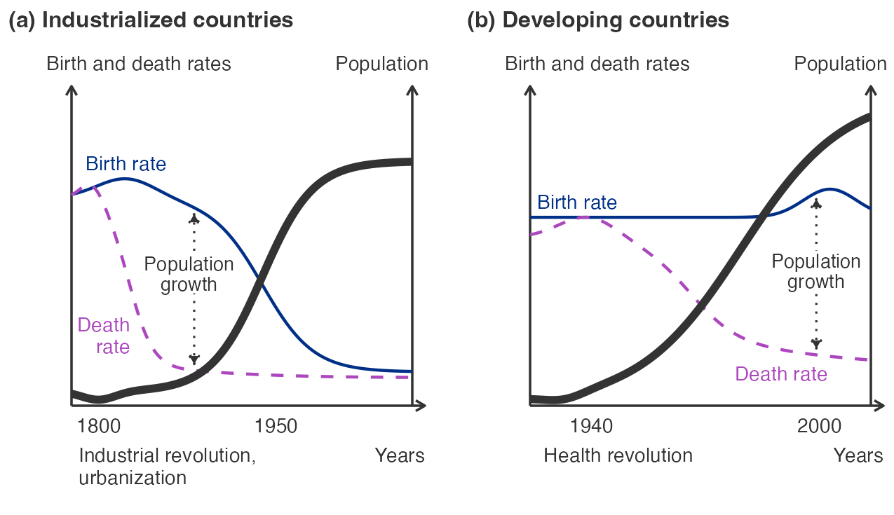
Population Pyramids and Dependency Ratios

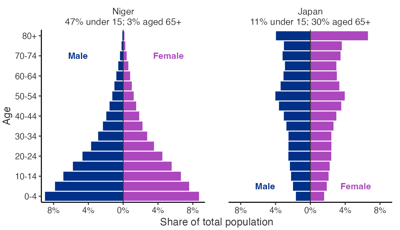
We might also use a population pyramid to represent population growth, birth rates, and death rates. A wide base represents a high birth rate while a narrow top represents a high death rate.

From the pyramid, we can observe a country’s dependency ratio: the non-working-age to working-age population (or specifically elder dependency ratio). When population growth is slow, this second ratio tends to be higher, where fewer young workers are supporting more older people (e.g. Japan).

Population Pyramids: Niger and Japan

Population by age and sex, 2024. World Bank, World Development Indicators

Population Growth: Too Slow and Too Fast

As a general fact, we now observe that population growth is too slow in many developed countries and too fast in many developing countries.

International migration could be a remedy to this, but such migration is now heavily restricted among many countries. As a result, we see surplus labor accumulate in some countries (e.g. India and other South Asian countries) while other countries face labor shortages (e.g. Japan, Germany, and other European countries).

Four Aspects of World Population

Four important aspects of world population:

1. Eighty-three percent of world population lives in LMICs²

2. World population is rapidly becoming urbanized while world poverty remains predominantly rural

3. LMICs include many megacities, high-density urban areas, e.g. Mexico City, Mumbai, São Paulo, Shanghai, Jakarta, and Lagos, where anti-poverty programs tend to be less successful than in rural areas

4. The population and economic costs from HIV/AIDS in sub-Saharan Africa are enormous (refuting Malthusian arguments, e.g. Young, 2005)

Economic Assumptions About Fertility

Economic assumptions about fertility decisions:

• Fertility outcomes are subject to willful choice by parents

• Fertility decisions are determined by the calculus of advantage, based off the income³, insurance⁴, and life satisfaction⁵ benefits children provide

• Methods of fertility control range in effectiveness and access is heterogeneous, such that the actual number of children may exceed the desired number for some households

The Quantity-Quality Tradeoff

If TFR falls with income, are children an inferior good⁶?

Not quite: intensive demand for children rises with income, but this includes demand for higher-quality and more costly children. Thus, extensive demand for children falls with income, as the number of children desired declines (Becker, 1981).

Galor (2010) also notes that technological change that increased demand for human capital accompanied the changing demand from child quantity to quality in the 19th century. More recently, availability of cheap and effective contraception has allowed parents to better control fertility and invest in child quality.

Various studies debate whether the decline in TFR is more due to demand side or supply side factors, e.g. changing tastes vs. availability of contraception (Miller, 2010; Rosenzweig, 1990).

Banerjee & Duflo on Contraception

The availability of contraception gives women more control over their reproductive lives—they can decide not just how many babies to have but also when to have them. And there is clear evidence that getting pregnant too early in life is very bad for the health of the mother. Moreover, early pregnancy, or even getting married, often results in dropping out of school.

— Banerjee & Duflo, pp. 121-122

Fertility and Externalities

Policy responses to TFR depend on whether children deliver positive or negative externalities to society: whether their social benefits are greater or less than their private benefits.

In the former case, governments may implement subsidies, while in the latter case, governments may implement taxes or other disincentives.

We could also consider the spillovers of one child to another. In many countries we observe a preference for boys and thus “missing women” (Sen, 1990). In others, this preference may lead to girls being in larger households than boys, as families have children until they have a boy, meaning girls have on average less access to household resources than boys (Jensen, 2003).

Banerjee & Duflo on Control over Fertility

[…] the answer to the question ‘Do the poor control their family decisions?’ thus seems to proceed in two steps. At the most obvious level, they do: their fertility decisions are the product of a choice, and even the lack of availability of contraception does not seem to be a big constraint. At the same time, what leads them to make these choices may be in part factors that are outside their immediate control: Women, in particular, may be pressured by their husbands, their mothers-in-law, or social norms to bear more children than they would like.

— Banerjee & Duflo, p. 129

Banerjee & Duflo on Population Policy

The most effective population policy might therefore be to make it unnecessary to have so many children (in particular, so many male children). Effective social safety nets (such as health insurance or old age pensions) or even the kind of financial development that enables people to profitably save for retirement could lead to a substantial reduction in fertility and perhaps also less discrimination against girls.

— Banerjee & Duflo, p. 141

5-minute Break

Ashraf, Field, & Lee (2014)

Randomly selected presenter: Ouly

1. What is the research question?

2. How do the authors answer it?

3. What do they find?

4. Are you convinced by the design and results?

5. How does the paper connect to our other readings?

de Janvry & Sadoulet on Ashraf, Field, & Lee

Ashraf et al. (2014) used an RCT in Zambia to test the usefulness of involving men in decision-making regarding the use of contraception. They contrasted a treatment where both husband and wife were offered access to injectable hormonal contraception with one where the offer was made to the woman alone (this form of contraception was observable only to the woman). They found that involving men reduced demand for contraception by 19 percent and increased the likelihood of giving birth by 27 percent. Allowing only women access to concealable contraception is thus a better approach to reducing fertility. They found, however, that this had a long-term cost for household harmony, with more mistrust and tension and lower happiness and health among women as a psychological cost of making contraceptives concealable. Giving some control to men over contraceptive decisions may thus lessen marital tensions created by the moral hazard of unobservable contraceptive methods.

— de Janvry & Sadoulet, p. 296

Group Discussion

Bringing together our lecture material and academic article, I have prepared the following suggested discussion questions:

• What are the implications of our different household bargaining models for various social policies, including cash transfers, work programs, and family planning?

• What are the demand-side and supply-side arguments for the decline in fertility as income rises? How do these relate to the quantity-quality tradeoff?

• We have previously discussed the Malthusian Trap, population tax, and dual-economy models of structural transformation. How do these relate to our discussion of the demographic transition and the fertility decline?

Roadmap

Looking Ahead to Week 8

What do we have on the horizon before next Tuesday?

• Our Literature Review assignment will be due on Friday at 6pm

• My office hours for ECON 672 will be held Tuesday before class, 12:15-2:15pm in MCL 108 or virtually by appointment

• Our eighth topic will be Financial services for the poor: credit and microfinance. Our textbook reading will be Chapter 13, pp. 326-338. Our Poor Economics reading will be Chapter 7. Our required journal article will be Banerjee, Duflo, Glennerster, & Kinnan (2015), “The Miracle of Microfinance?” AEJ: Applied.

• Our Weekly Reading Response assignment for this paper will be due Tuesday at 2:40pm before class. One student will be randomly selected to present their response to the class in 5-8 minutes.

Footnotes

1. Ethiopia’s last completed census was in 2007: the UN estimates 132 million people, Ethiopia’s own statistical service 108 million. On the smaller count, GDPpc would be about 22% higher.

2. World Bank, World Development Indicators, 2024.

3. When children work in fields or factories, their wages are contributed to household income.

4. A large number of children allows a household to diversify its sources of income for risk management, receive transfers from children for risk coping following a shock, provide physical protection to parents, and offer them old-age protection.

5. Children can be seen as a durable consumer good, with tradeoffs for the household between the quantity and quality of children.

6. An inferior good is one with a negative income elasticity of demand, such that demand falls as income rises. This is opposite of a normal good with a positive income elasticity of demand, where demand moves with income.